Seigyo kogaku shuho o mochiita sapuraichen pafomansu hyoka hoho ni kansuru kenkyu

Performance Measurement of the Supply Chain Using Control Engineering Approach. September 2015. Mohammadreza Parsanejad.

Performance Measurement of the Supply Chain Using Control Engineering Approach. by Mohammadreza Parsanejad. Submitted in Partial Fulfillment of the Requirement for the Degree of Doctor of Engineering September 2015. Dissertation supervisor Professor Hiroaki Matsukawa. Department of Administration Engineering Graduate School of Science and Technology Keio University.

Abstract A supply chain is an integrated process wherein raw materials are extracted and converted to the final products, and delivered to the customer. To design and analyze an appropriate supply chain we have to evaluate its performance. In practice, performance measurement of the supply chain is complicated due to the influence of different parameters involved in production planning, inventory control, logistics and transportation activities through the chain. On the other hand control theory is a well-known methodology to measure performance of business related problems. In control theory differential equations of a continuous model is derived in time domain and then Laplace transform is used to convert the model to the complex frequency domain or simply s-domain. The converted model is solved and the solution converted back to time domain by invers Laplace transform. The purpose of this dissertation is to measure performance of the supply chain using frequency response analysis. So control theory approach is used to measure different performance aspects of the supply chain. The IOBPCS model is used as a benchmark to propose an analytical approach for modelling production smoothing constraints. Since production constraints are nonlinear, the extended model which in this research is called Nonlinear IOBPCS (NIOBPCS) is no longer linear and thus nonlinear control theory is applied to measure frequency response for zero target inventory. The results of frequency response show improvement of production performance of the system facing with production smoothing constraints compared with the system without constraints, but deterioration of inventory performance especially if demand has higher amplitudes so amplitude of production signal ideally should be more than production constraints but practically could not be fluctuate appropriately to satisfy the customer demand. Due to lower performance of inventory in zero target inventory condition stock outs is observed during demand peaks, so non-zero target inventory conditions is applied to calculate the amount of safety stock that is necessary to have no stock out in the supply chain. Furthermore a total performance function is developed based on APIOBPCS which is an extended version of IOBPCS. Frequency response is used to introduce a total performance function encompassing all types of the system costs including production, finished goods holding and shortage, WIP, and ordering costs. The developed total performance function represents aggregate performance of the system in one general function. The results of sensitivity analysis of total performance function indicate a reverse effect of work in process recovery speed compared with finished goods recovery and demand updating rate for different demand frequencies.. i.

In the name of God.. ii.

Notation IOBPCS: Inventory and Order Based Production and Inventory System APIOBPCS: Automotive Pipeline Inventory and Order Based Production and Inventory System s:. Laplace operator :. t:. Demand frequency Time. T: D: P: I:. Time period Demand Production Finished goods inventory. WIP:. Work in process inventory Maximum value of demand signal Maximum value of production signal. : : : | / | | / | | / | : : : :. Maximum value of finished goods inventory Maximum value of work in process inventory Maximum value of demand signal Amplitude ratio of production to demand Amplitude ratio of Inventory to demand Amplitude ratio of WIP to demand Production lead time Estimated production lead time. : TINV: TWIP: EINV: EWIP:. Time to adjust finished goods inventory Time to adjust demand Time to adjust WIP Target level of finished goods Target level of WIP Error of finished goods Error of WIP. L: W:. Average number of items in the system Average waiting time of an item. λ:. Throughput of the system Product cost per unit Production variation cost per unit Finished goods holding cost per unit. iii.

Shortage cost per unit WIP excess cost per unit Ordering cost per order. iv.

Contents Abstract .............................................................................................................................. i Notation ........................................................................................................................... iii List of Figures ................................................................................................................. vii 1. Introduction .............................................................................................................. 1 1.1 Research motivation ........................................................................................... 1 1.2 Research scope ................................................................................................... 3. 1.3 Thesis structure ................................................................................................... 4 2 Methodology............................................................................................................. 6 2.1 Laplace transform ............................................................................................... 6 2.1.1 Definition ..................................................................................................... 7 2.1.2 2.2. Properties of Laplace transform .................................................................. 8. Convolution ...................................................................................................... 10. 2.3 Inverse Laplace ..................................................................................................11 2.4 Transfer function .............................................................................................. 12 2.4.1 Definition of Transfer function .................................................................. 12 2.4.2. Order of transfer functions ........................................................................ 13. 2.4.3. Inputs of transfer function ......................................................................... 13. 2.4.4. Integrator ................................................................................................... 15. 2.4.5. First order transfer function ....................................................................... 19. 2.4.6. Second order transfer function .................................................................. 22. 2.5 Block diagram .................................................................................................. 31 2.5.1 Block diagram reduction ........................................................................... 31 2.5.2. Open and closed loop systems ................................................................... 33. 2.6 Frequency response .......................................................................................... 35 2.6.1 Gain ........................................................................................................... 37. 3. 2.6.2. Integrator and derivative............................................................................ 39. 2.6.3. Double integrator and derivative ............................................................... 41. 2.6.4. Zero and pole ............................................................................................. 43. 2.6.5. Second order transfer function .................................................................. 45. Literature review..................................................................................................... 49. v.

3.1. IOBPCS family ................................................................................................. 54. 3.2 3.3 3.4 3.5. IOBPCS ............................................................................................................ 55 IBPCS ............................................................................................................... 59 OBPCS ............................................................................................................. 61 VIOBPCS ......................................................................................................... 64. 3.6 VIBPCS ............................................................................................................ 66 3.7 APIOBPCS ....................................................................................................... 68 4 Nonlinear IOBPCS (NIOBPCS)............................................................................. 71 4.1 4.2 4.3 4.4. Introduction ...................................................................................................... 71 Control theory and nonlinearity........................................................................ 72 Modelling production smoothing ..................................................................... 73 Nonlinear control theory................................................................................... 76. 4.5 Frequency Response of NIOBPCS ................................................................... 78 4.6 Analysis of results ............................................................................................ 84 4.7 NIOBPCS with Non-zero Target inventory ...................................................... 85 5 Total performance function .................................................................................... 89 5.1 Introduction ...................................................................................................... 89 5.2 Overview .......................................................................................................... 90 5.3 Response of the system .................................................................................... 91 5.4 Parameter adjustment ....................................................................................... 95 5.5 Defining total performance function ................................................................ 97 5.5.1 Production performance ............................................................................ 97. 6. 5.5.2. Finished goods holding and shortage performance ................................... 97. 5.5.3. WIP excess and starvation performance .................................................... 98. 5.5.4. Ordering performance................................................................................ 98. 5.5.5. Integrated formula ................................................................................... 100. Conclusion ............................................................................................................ 104 6.1 Summary......................................................................................................... 104 6.2 Future research opportunities ......................................................................... 105. References .................................................................................................................... 107 Appendix A: Laplace transform table............................................................................113 Appendix B: Frequency response ..................................................................................118 Appendix C: Ellipses .................................................................................................... 120 Acknowledgements ...................................................................................................... 121. vi.

List of Figures Figure 1.1 Supply chain Models. .............................................................................. 3 Figure 1.2 Supply chain Modelling .......................................................................... 3 Figure 2.1 Laplace transform.................................................................................... 6 Figure 2.2 Inverse Laplace transform ....................................................................... 7 Figure 2.3 Transfer function of a system, its input and output ............................... 12 Figure 2.4 Unit input .............................................................................................. 13 Figure 2.5 Ramp input ............................................................................................ 14 Figure 2.6 Impulse input ......................................................................................... 14 Figure 2.7 Integrator transfer function ................................................................... 15 Figure 2.8 Output of the integrator for step input................................................... 16 Figure 2.9 Output of the integrator for impulse input ............................................ 17 Figure 2.10 Output of the integrator for ramp input ............................................... 18 Figure 2.11 First order transfer function................................................................. 19 Figure 2.12 Output of the first order function for step input .................................. 19 Figure 2.13 Output of the first order function for impulse input............................ 20 Figure 2.14 Output of the first order function for ramp input ................................ 21 Figure 2.15 Second order transfer function ............................................................ 22 Figure 2.16 Pole movement .................................................................................... 22 Figure 2.17 Output of the second order function for step input with Figure 2.18 Output of the second order function for step input with Figure 2.19 Output of the second order function for step input with. = 0.......... 23 = 0.1....... 24 = 1.......... 24. Figure 2.25 Output of the second order function for ramp input with Figure 2.26 Output of the second order function for ramp input with Figure 2.27 Output of the second order function for ramp input with. = 0 ........ 28 = 0.1 ..... 29 = 1 ........ 29. Figure 2.20 Output of the second order function for step input with = 3.......... 25 Figure 2.21 Output of the second order function for impulse input with = 0 ... 26 Figure 2.22 Output of the second order function for impulse input with = 0.1 26 Figure 2.23 Output of the second order function for impulse input with = 1 ... 27 Figure 2.24 Output of the second order function for impulse input with = 3 ... 27 Figure 2.28 Output of the second order function for ramp input with = 3 ........ 30 Figure 2.29 Block diagram reduction ..................................................................... 32 Figure 2.30 Open loop system ................................................................................ 33 Figure 2.31 Closed loop system ............................................................................. 33 Figure 2.32 Open loop system without taking into account disturbances .............. 34. vii.

Figure 2.33 Open loop system with taking into account disturbances ................... 34 Figure 2.34 Closed loop system without taking into account disturbances ........... 34 Figure 2.35 Closed loop system with taking into account disturbances................. 34 Figure 2.36 Pattern of daily electricity usage Tokyo area ...................................... 35 Figure 2.37 Bode diagram of G(s) =2 .................................................................... 38 Figure 2.38 Bode diagram of G(s) =-5 ................................................................... 38 Figure 2.39 Bode diagram of G(s) =s ..................................................................... 40 Figure 2.40 Bode diagram of G(s) =1/s .................................................................. 40 Figure 2.41 Bode diagram of Figure 2.42 Bode diagram of Figure 2.43 Bode diagram of Figure 2.44 Bode diagram of. G(s) = s2................................................................. 42 G(s) = 1/s2 ............................................................. 42. G(s) = 2s + 1 .......................................................... 44 G(s) = 1/(2s + 1) ................................................... 44. Figure 2.45 Bode diagram of G(s) = 1/(s2 + 9) ................................................... 45 Figure 2.46 Bode diagram of G(s) = 1/(s2 + 2s + 2) ........................................... 46 Figure 2.47 Bode diagram of G(s) = 1/(s + 2)2 ................................................... 47 Figure 2.48 Bode diagram of G(s) = 1/(%2 + 5s + 6)............................................ 48 Figure 3.1 Supply chain activities .......................................................................... 49 Figure 3.2 Supply chain processes ......................................................................... 50 Figure 3.3 Structural dimensions of the supply chain ............................................ 51 Figure 3.4 Material and information flows ............................................................. 51 Figure 3.5 Supply chain interdependences ............................................................. 52 Figure 3.6 Supply chain Models ............................................................................. 53 Figure 3.7 Supply chain Modelling ........................................................................ 53 Figure 3.8 The IOBPCS family. ............................................................................. 54 Figure 3.9 Block diagram of IOBPCS .................................................................... 55 Figure 3.10 Response of IOBPCS to Demand=unit step and TINV=0 .................. 57 Figure 3.11 Response of IOBPCS to Demand=unit impulse and TINV=0 ............ 57 Figure 3.12 Response of IOBPCS to Demand=sin(0.3t) and TINV=0 .................. 58 Figure 3.13 Response of IOBPCS to Demand=0 and TINV=5 .............................. 58 Figure 3.14 Block diagram of IBPCS..................................................................... 59 Figure 3.15 Response of IBPCS to Demand=unit step and TINV=0 ..................... 59 Figure 3.16 Response of IBPCS to Demand=unit impulse and TINV=0 ............... 60 Figure 3.17 Response of IBPCS to Demand=sin(0.3t) and TINV=0 ..................... 60. Figure 3.18 Response of IBPCS to Demand=0 and TINV=5................................. 61 Figure 3.19 Block diagram of OBPCS. .................................................................. 61 Figure 3.20 Response of OBPCS to Demand=unit step and TINV=0 ................... 62. viii.

Figure 3.21 Response of OBPCS to Demand=unit impulse and TINV=0 ............. 62 Figure 3.22 Response of OBPCS to Demand=sin(0.3t) and TINV=0 ................... 63 Figure 3.23 Response of OBPCS to Demand=0 and TINV=5 ............................... 63 Figure 3.24 Block diagram of VIOBPCS. .............................................................. 64 Figure 3.25 Response of VIOBPCS to Demand=unit step and TINV=0 ............... 65 Figure 3.26 Response of VIOBPCS to Demand=unit impulse and TINV=0 ......... 65 Figure 3.27 Response of VIOBPCS to Demand=sin(0.3t) and TINV=0 ............... 66 Figure 3.28 Block diagram of VIBPCS. Source: Lalwani et al. (2006) ................. 66 Figure 3.29 Response of VIBPCS to Demand=unit step and TINV=0 .................. 67 Figure 3.30 Response of VIBPCS to Demand=unit impulse and TINV=0 ............ 67 Figure 3.31 Response of VIBPCS to Demand=sin(0.3t) and TINV=0 .................. 68 Figure 3.32 Block diagram of APIOBPCS. ............................................................ 68 Figure 3.33 Response of APIOBPCS to Demand=unit step, TINV=0 ................... 69 Figure 3.34 Response of APIOBPCS to Demand=unit impulse, TINV=0 ............. 69 Figure 3.35 Response of APIOBPCS to Demand=sin(0.3t), TINV=0 ................... 70 Figure 3.36 Response of APIOBPCS to Demand=0, TINV=5............................... 70 Figure 4.1 Three types of production system. ........................................................ 74 Figure 4.2 Illustration of the production smoothing constraints ............................ 74 Figure 4.3 Block diagram of IOBPCS and NIOBPCS. .......................................... 75 Figure 4.4 Block diagram of the reconfigured NIOBPCS ..................................... 75 Figure 4.5 Intersection of left and right sides of Eq (7) for M=1 and w=0.4 ......... 77 Figure 4.6 Left and right sides of Eq(7) for M=0.6 and w=0.1,0.2,0.3,0.4,0.5. ..... 79 Figure 4.7 Left and right sides of Eq(7) for M=2 and w=0.1,0.2,0.3,0.4,0.5 ......... 79 Figure 4.8 P/D amplitude ratio. .............................................................................. 80 Figure 4.9 Normal and Cutting area of NIOBPCS ................................................. 81 Figure 4.10 Simulation results of NIOBPCS ......................................................... 82 Figure 4.11 I/D amplitude ratio .............................................................................. 83 Figure 4.12 Response of NIOBPCS for TINV=0 and 6.57 .................................... 87 Figure 4.13 Inventory holding and stock out for TINV=2 ..................................... 88 Figure 5.1 Block diagram of APIOBPCS in S-Domain ......................................... 91 Figure 5.2 Correspondences between WIP,Tp, P in APIOBPCS, and L, λ, W....... 93 Figure 5.3 Frequency response of production, finished goods, WIP and order ..... 94 Figure 5.4 Impact of different parameter settings on the system performance ...... 96 Figure 5.5 Production, finished goods and WIP levels........................................... 99 Figure 5.6 Total performance ............................................................................... 101 Figure 5.7 Total performance sensitivity .............................................................. 102. ix.

1 Introduction 1.1 Research motivation A supply chain is a network of companies involved at upstream and downstream of a chain involving at different activities and processes to deliver product to the hand of end customer (Christopher, 1992). The supply chain takes into account all processes of production and processing from raw material to delivery of final product (New & Payne, 1995). So in the supply chain there is an integrated process wherein raw materials are extracted and converted to the final products, and delivered to the customer where processes could be divided to upstream and downstream processes. The upstream processes consist of production planning and inventory control including manufacturing and holding of sub processes. The aim of these processes are design ,management and control of a production planning, scheduling and acquisition system for all materials including raw material, work in processes and finished goods. But downstream processes on the other side are about distribution and logistics process and concentrate on the transportation of the final products to the end customer through retailers or sometimes to the wholesalers. These processes include design, management and control of logistic activities at downstream of the supply chain until the end customer (Beamon, 1998). Furthermore every supply chain has different flows up to down and vice versa through the chain. One of the most important flows is material flow which could be considered almost up to downstream. Existence of recycling or reuse paths create another material flow but from down to upstream. Generally material flow includes acquisition of raw materials and parts which then will be processed and added values until the end consumer (Cooper et al., 1997). Another important flow through the supply chain is information flow which should not be neglected from our analysis. The information flow has reverse direction compared with material from such that information is down to upstream from customer to the retailer. The retailer in tune makes an order based on the consumers’ order and send it up to the warehouse or distributer. And distributer gathers all retailers’ orders, sum it up, then place an order based on its current stock, customer demand and forecasting method. Now the order is on the production line where manufacturer should produce the final product necessary to satisfy the down stream’s demand. To follow demand the manufacturer have to supply raw material to build and assemble them and deliver it to the downstream. So in order to complete the whole chain, another order is necessary from manufacturer to the suppliers (Min & Zhou, 2002).. 1.

As it is clear performance measurement of a supply chain with above-mentioned characteristics is complicated due to the impact of a variety of factors parameters involved in a wide range of activities such as production planning, inventory control, logistics and transportation through the whole supply chain. In order to design and analyze an appropriate supply chain we have to evaluate its performance to observe the present situation of the chain. On the other hand control theory is a well-known methodology to measure performance of engineering, economics and also business related problems. Control theory uses transformed version of the problem to overcome complexity issues. In control theory first differential or difference equations of a model is written in time domain. These equations shows behavior of one phenomena or the whole system over time. After deriving model equations in time domain, Laplace transform is used to convert the continuous model to the complex frequency domain or simply s-domain. In case of discrete model z-transform is applied to derive the converted version of model. The converted model is solved in the transformed domain and the solution converted back to time domain. For continuous model invers Laplace transform is used to return the solution to the time domain and for discrete model the inverse z-transform is applied for this operation. Control theory has a variety of advantages compared with dealing with the problem in time domain. The problem often become simpler to solve after converting to equation transformed domain. For instance differential equations converts to algebraic equations (Dorf & Bishop, 2010). Moreover since the transformed version of the model automatically include initial conditions therefore both steady state and transient solution could be analyzed altogether (Ogata, 2004). The converted version of the problem is often easy to solve compared with its original form and could be solved in the transformed domain and then the solution is again reconverted to the original domain using invers Laplace transform. And also for signals that are physically realizable we always could find their Laplace transforms (Dorf & Bishop, 2010). In practice models representing supply chain activities are complicated and include more than only one difference or differential equation. In this situation still control theory could be applied because not only a single function but also a set of interconnected differential or difference equations with its accompanying initial values could be converted to the transform version and solved then reverted to the original format by inverse transform operators. So by using control theory we have capability to transfer a whole model consisting of multiple differential equations to s-domain. In this research the control theory is applied to measure and evaluate the performance of a supply chain including production, inventory and work in process.. 2.

1.2 Research scope Supply chain models generally categorized into deterministic and stochastic models (Beamon, 1998). But there are also other detailed categorizations. Min & Zhou (2002) in a comprehensive literature review about supply chain modelling discover four different types of supply chain models including deterministic, stochastic, hybrid and IT-driven models. They divide deterministic models to single and multiple objectives, stochastic models to optimal control theory and dynamic programing, hybrid models to inventory theoretic and simulation, and IT-driven models to WMS, ERP and GIS as illustrated in Figure 1.1.. Figure 1.1 Supply chain Models. Source: Min & Zhou (2002) And since supply chains have always cross functional properties, Min & Zhou (2002) define integrated supply chain modeling only if they take into account different functions of the supply chain together. They specifically categorize integrated supply chain modelling into five different categories consisting of supply selection/ inventory control, production/ inventory, location/ inventory control, inventory control/ transportation as shown in Figure 1.2.. Figure 1.2 Supply chain Modelling Source: Min & Zhou (2002) On the other hand supply chain is a phenomena which we could write its differential equations in time domain. And similar to other physical and natural phenomena we could convert supply chain differential equations to the s-domain using Laplace transformation.. 3.

Therefore we could deal with a supply chain problem both in time and s-domain. In this study we aim to model a typical continuous supply chain in s-domain and then measure its performance and analyze its behavior for different deterministic demand fluctuations. Based on this argument our study fits to the category of deterministic models with multiple objectives in Figure 1.1 and our modelling approach falls into the category of production/inventory or inventory control/transportation approaches in Figure 1.2. 1.3 Thesis structure The aim of this dissertation is to evaluate performance of a continuous deterministic supply chain using control theory and more specifically frequency response analysis. Therefore after introducing research motivation and scope in chapter 1, we focus on analysis of control theory principles as a basis for our modelling and design in chapter 2. In chapter 2 applications of control theory is explained and then Laplace transform as an important approach in this field is demonstrated. Laplace transform is defined and number of its properties of Laplace transform indicated such as linearity, s shifting, time shifting, integration, differentiation, initial and final value theorems. Then the convolution integral as the based for Laplace transform is demonstrated. And finally the last step of Laplace transform analysis i.e. inverse Laplace transform is explained in chapter 2. Laplace transform is used to make transfer functions. Therefore in chapter 3, transfer function analysis is discussed. First a transfer function is define and then order of typical transfer functions is explored. In order to understand transfer function analysis we have to know what would be the response of a transfer function to different inputs. Thus the response of integrator, first order transfer function and second order transfer function to constant, step, impulse and ramp inputs are analyzed. The higher level of analysis is to analyze a whole system. In order to analyze the whole system we have to make the block diagram of the whole function of the system including all interconnected phenomena in the format of block diagram. Therefore in chapter 4, block diagram analysis is demonstrated and then block diagram reduction as a basic method for deriving transfer function of the system is explained. And finally open and close loop block diagrams is indicated at the end of chapter 4. Transfer function and block diagram analysis are principles of deriving frequency response of the system. After block diagram reduction and deriving transfer function of the system we have to find frequency response of the most important signals of the system. Therefore frequency response of gain, integrator and derivative, double integrator and derivative, second order transfer function with different damping ratios from zero to infinity is derived and demonstrated in chapter 5.. 4.

After analyzing control theory, Laplace transform and block diagram we demonstrate supply chain most important features including supply chain activities, supply chain processes, structural dimensions of the supply chain, material and information flows, supply chain interdependences, supply chain models and supply chain modelling in chapter 6. After analysis of different supply chain features we have to focus on control theoretic models that have already been developed in previous studies. Since the main goal of this research is concentrated on IOBPCS family, at continuation of chapter 6 this modelling approach is demonstrated. Although there are different versions of IOBPCS but in this chapter the transfer functions of production, finished goods inventory, work in process inventory are derived only for Inventory and Order Based Production and Inventory System (IOBPCS), Inventory Based Production and Inventory System (IBPCS), Order Based Production and Inventory System (OBPCS), Variable Inventory and Order Based Production and Inventory System (VIOBPCS), Variable Inventory Based Production and Inventory System (VIBPCS) and Automotive Pipeline Inventory and Order Based Production and Inventory System (APIOBPCS). And finally response of the system to step, impulse and sinusoidal demand subject to zero and non-zero target inventories are analyzed. Since IOBPCS model is used as a benchmark for our study it is utilized to model production smoothing constraints in chapter 7. Production smoothing constraints are nonlinear phenomena, resulting in the extended model which in this research is called Nonlinear Inventory and Order Based Production and Inventory System (NIOBPCS) is no longer linear. Therefore we have to apply nonlinear control theory to measure frequency response and evaluate its performance. First the response of NIOBPCS to zero target inventory is analyzed and then the non-zero target inventory conditions is applied to calculate the amount of safety stock that is necessary to have no stock out or less levels of stock out in the supply chain. Furthermore a total performance function based on APIOBPCS which is an extended version of IOBPCS considering work in process inventories, is developed in chapter 8. The frequency response is utilized to introduce a total performance function encompassing all types of the system costs including production, finished goods holding and shortage, WIP excess and starvation, and ordering costs. The developed total performance function represents aggregate performance of the system in one general function enabling us to analyze total performance of the supply chain as a whole system. In chapter 9 we conclude the research by a summary and an outlook of the result, plus a brief discussion for future researches.. 5.

2 Methodology In this study control theory is applied as methodology of the research. The control theory deals with analysis and design of computer control and management system or decision support systems, to construct decision making algorithms needed for such systems (Bubnicki, 2005, p.1). Control theory has a wide range of applications in industry, economics, finance, marketing, natural resources, maintenance and replacement, distributed systems, production and inventory control (Sethi & Thompson, 2000, p.1). It is also applied to intelligent systems such as machine tools, flexible robotics, photolithography, biomechanical and biomedical, and process control (Golnaraghi & Kuo, 2010, p.2). Development of control systems backs to 1769 when 1769 James Watt's made first steam engine and governor to mark the beginning of the Industrial Revolution (Dorf & Bishop, 2010, p.9). Since then control theory has used in different control system in order to produce necessary needs of human being in the industrial ages. Laplace transform has an important role in the design and modelling of the system using control theory and the aim of this section is to establish a comprehensive context for analyzing performance of the supply chain based on Laplace transform. 2.1 Laplace transform Mathematical transforms are operators converting functions from one space to the other. Laplace transform is a well-known operator that is applicable in a wide range of engineering and science including differential equations, control engineering, communication, signal processing and system analysis. The Laplace transform converts functions to the complex frequency or simply s-domain as shown in Figure 2.1 where the Laplace transform is shown with L, the original function with f(t) and the converted function with F(s).. L[f(t)]=F(s) f(t). F(s). t-domain. s-domain Source: Dyke (2014) p.3 Figure 2.1 Laplace transform. 6.

In the field of operation research we often transform functions from time domain such as inventory, production or order functions over time to s-domain to analyze the system behavior. . After converting to s-domain, the problem often become simpler to solve. For instance differential equations converts to algebraic equations (Dorf & Bishop, 2010) or since the transformed form automatically include initial conditions therefore both steady state and transient solution could be analyzed altogether (Ogata, 2004, p.14). The converted version of the problem is often easy to deal compared with its original form and could be solved in the s-domain and then the solution is again reconverted to the original domain using invers Laplace transform as shown in the Figure 2.2. For signals that are physically realizable we always could find their Laplace transforms (Dorf & Bishop, 2010). Not only a function but a whole differential equation with its accompanying initial values could be converted to the s-domain and solved then reverted to the original format by inverse Laplace transform. Furthermore the Laplace transform has capability to transfer a whole model consisting of multiple differential equations to s-domain. In this situation which we are looking for, first the whole model is developed in time domain and then converted to s-domain.. Inverse Laplace transform f(t). F(s). t-domain. +3 ,*(%)/ = -(.). s-domain. Figure 2.2 Inverse Laplace transform 2.1.1 Definition Given the desired function of f(t) in time domain, its Laplace equivalent is defined as (cf. Churchill, 1958). 7. *(%) = +,-(.)/ = 1 2 345 -(.)6. 8. where L is Laplace operator, t is time variable from zero to infinity, s is complex frequency, f(t) is desired function in time domain and F(s) is converted version of f(t) in s-domain. 7.

And s is the complex frequency which includes imaginary and real parts is defined as below:. s = σ + jω, where σ, ω are real numbers and i is imaginary unit defined as. j = √−1. There are other definitions of Laplace transform. Eq(1) is one side or unilateral Laplace transform but the two side or bilateral transform which is more close to Fourier transfer is defined as (cf. Oppenheim et al., 1997). *(%) = +,-(.)/ = >37 2 345 -(.)6. 7. This equation is used in mathematics and probability theory but in our study the main variable of almost all inputs and outputs of an inventory production system is time, and since negative time does not have meaningful concept in operation research we use oneside Laplace transform to covert system signals such as inventory and production and moreover differential equations of the system. 2.1.2 Properties of Laplace transform A comprehensive Laplace transform table is proposed in Appendix A, but here some of its special specifications that facilitate its applicability in different problems with different conditions is explained. In this section we introduce some of its properties that could be applied in the modelling of production and inventory system (cf: Dyke, 2014) 2.1.2.1 Linearity If f(t) and g(t) are two functions that their Laplace transforms exist, then their weighted summation also have Laplace transform as below. +,?-(.) + @A(.)/ = ?+,-(.)/ + @+,A(.)/ = a*(%) + @C(%), where F(s) and G(s) are Laplace transforms of f(t) and g(t), and a and b are two arbitrary constant numbers. 2.1.2.2 s shifting The Laplace transform have two shifting properties. The first shifting happens on transformed side where F(s), the Laplace transform of f(t) shifts by a constant number as below: +,2 3 5 -(.)/ = *(% + ?). The effect of shifting in transformed side is a multiplying component i.e. e3EF , on the t 8.

side. 2.1.2.3 Time shifting The second shifting property is on the original side where the function in time domain. shifts by a constant number 0 ≤ ? as below: +,-(. − ?)/ = 2 3 4 *(%) This property is significantly important for us since it could represents the substantial lead time phenomena in production and inventory systems (Grubbstrom & Tang, 2000). For instance if production line have the lead time of Tp, then there would be a time delay between placing an order and delivery of the final product. In this case the transfer function that connects order to delivery is:. Delivery(s) = e3EN OP62P(%) This equation shows a transfer function between delivery and order of a production system. It means that the delivery rate is a function of order rate but with a pure delay that indicates the lead time of the production line. We will later comprehensively explain what is transfer function and how it works in our modeling in detail. 2.1.2.4 Integration If L[f(t)]= F(s), then we will have:. +,>8 -(Q)6Q/ = 5. R(4) 4. ,. where τ is an artificial variable only for doing the integral operation. This property has many applications in our modelling and everywhere that we have an integrational phenomena. It could be used to figure out the transfer function of the operation in sdomain. For instance inventory in all of its shapes including finished goods or work in process, have integral properties such that it accumulates over time and makes inventory position. We will use the basic of this property in different situations in the modelling of our inventory production system in the next sections. 2.1.2.5 Differentiation The Laplace of a differentiation function could be derived through its Laplace transformation as below: U V = %*(%) − -(0), +T-(.). where F(s) is the transformed version of f(t). This equation shows that the Laplace transformation of differentiation of a function is not only a function of Laplace of the original function but also to its initial conditions.. 9.

The second differentiation of f(t) also could be calculated by its Laplace transformation as below:. X V = % *(%) − %-(0) − -U (0) LT-(.). 2.1.2.6 Initial value The Initial value theorem allows us to find the value of desired signal at t=0 based on its transformed version as below lim -(.) = lim %*(%), 5→8. 4→7. where F(s) is Laplace transform of f(t). 2.1.2.7 Final value On the other hand the final value theorem is used to analyze the function in the infinity which is utilized for analysis of steady state response of the system when system becomes stable as below lim -(.) = lim %*(%).. 5→7. 4→8. 2.2 Convolution The convolution of two functions is derived from integral of reverse of one the functions shifting over another function to produce a third function which is blending of two original function. (Hirschman & Widder, 1955). The convolution of two functions is denoted by f*g and calculated as below: (- ∗ A)(.) = >37 -(Q)A(. − Q) 6Q, 7. or since either of two functions could be inversed and shifted we could write the integral in another equivalent format as below (- ∗ A)(.) = >37 A(Q)-(. − Q) 6Q. 7. The convolution integral which has a significant role in the control theory is also known as Duhamel's integral or the Duhamel's Convolution Principle in mathematics and engineering (Shmaliy, 2007, p.154). The convolution integral has some properties that could help us in the further calculations and modelling. A set of convolution properties are as below (cf: Bracewell, 1965): f∗g= g∗f 10.

- ∗ (A ∗ ℎ) = (- ∗ A) ∗ ℎ - ∗ (A + ℎ) = (- ∗ A) + (- ∗ ℎ) ?(- ∗ A) = (?-) ∗ A = - ∗ (?A) (- ∗U A) = -U ∗ A = - ∗ AU ,. where a is an arbitrary constant number and f, g and h are integrable over time (Stein & Weiss 1971). The concept of convolution is fundamentally important in our modelling and analysis. The reason is behind the input-output analysis and the fact that finding output of the system in the time domain is hard and we need to sometimes convert the problem to the s-domain. But the output of the system will change for different input so we need to find a general method to overcome this difficulty. And convolution integral have the below characteristics that facilitate this problem:. +,-(.) ∗ A(.)/ = *(%)C(%) This property which is another significant underlying property of Laplace transform, allow us to find the convolution of two signals by just multiplying their corresponding transformed versions in s-domain. In our transfer function analysis there are many situations that we have to find the convolution of two signals, but since finding convolution integral is a time consuming process we simply replace it by the multiplication of Laplace of input and transfer function of the corresponding block. Indeed the concept of convolution integral is mostly useful in finding transfer function of each production-inventory phenomena and afterward making the block diagram of the whole system. In the next step we explain the concept of transfer function in detail. 2.3 Inverse Laplace The inverse Laplace is used to convert back the solution of a transformed version of a system, to the initial time domain. And virtually Laplace transform such as other operations has inverse and Laplace transform is not exception (Dyke, 2014, p.3). The inverse Laplace transform is expressed as below -(.) = +3 ,*(%)/(.) =. ab 7 45 2 *(%)6% > _` a3 7. , 0<t. where f(t)=0 at t<0, and integration is performed along the line s=c+jy in complex splane, while c is chosen so that s=c lies on the right of F(s) poles (Enns, 2006, p.244).. 11.

2.4 Transfer function Laplace transform has many applications in the solving electrical circuits or differential equations, and could be applied for a variety of problem from space control to economical and managerial problems. Application of Laplace transform in transfer function analysis via convolution integral are frequently used to explore the input-output relationship in components and whole systems. 2.4.1 Definition of Transfer function A transfer function is defined as the ratio of Laplace transform of the output to Laplace transform of Input with zero initial conditions (Ogata, 2004, p106). Assuming x(t) and y(t) as input and output of a system, and X(s) and Y(s) as their Laplace transformations respectively as shown in the Figure 2.3, the transfer function of the system with zero initial condition is calculated as below. P?c%-2P -dce.fgc = C(%) = = j(4). i(4). +(gd.hd.) +(fchd.). Having the transfer function we could easily find the output for any input of the system where we have. k(%) = l(%) × C(%). This is very important for us to model and observe the behavior of the system. Finding transfer function of a system has many advantageous for design, control and optimization of the system. X(s). Y(s) G(s). Figure 2.3 Transfer function of a system, its input and output The transfer function shows inherent properties of a system or component and in case of unknown transfer function, control engineers try to find it experimentally by introducing a set of known inputs and observing the corresponding outputs. Once the transfer function Figured out, it could be applied for any inputs (Ogata, 2004, p 107). In this approach the objective of control engineering is to control the outputs subject to specific inputs through controllers of the model to satisfy predefined objective of the system design (Golnaraghi & Kuo, 2010).. 12.

2.4.2 Order of transfer functions The transfer function of a single input single output linear time invariant system could be generally written in the form of C(%) =. nop 4 op b⋯bnr 4bnp. 4o b. osr 4. osr b⋯b. r 4b p. c ≤ c8 ,. where ?t3 , … , ?8 and @tp , … , @8 are real numbers, representing coefficients of. denominator and nominator, respectively. In this general equation n is the order of. denominator and also the order of whole system, and c8 is the order of nominator (Orlov & Aguilar, 2014, p.5). Since we use first and second order transfer function many times in our modelling, we investigate the behavior of some examples of first and second order systems subject to some fundamental inputs including step, impulse, ramp and sinusoid. But first we need to find Laplace transform of each of these inputs. 2.4.3 Inputs of transfer function The step input could represents turning on a system by switching on the key instantaneously (Sundararajan, 2008, p33). Considering the step function wd(.) =. 0 . < 0, w 0 < ., where A is a constant number and is shown in Figure 2.4. Au(t) A. 0. t. Figure 2.4 Unit input The parameter A could be shown as an exponential function with the power of zero. w = w2 5 , where a=0. So Laplace transform of a unit step function is (Ogata, 2004, p16) +,d(.)/ = >8 w 2 345 6. = 4 . 7. 13. y.

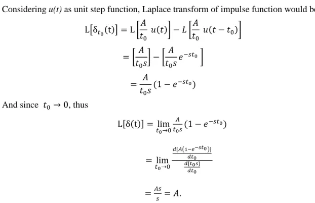
The ramp input could be shown as. P(.) =. 0 . < 0,. w. 0 < ., where A is constant number (Ogata, 2004, p17) and is shown in Figure 2.5. r(t) At. 0. t Figure 2.5 Ramp input. And its Laplace transform is. +,P(.)/ = >8 w. 2 345 6. = 7. y. 4z. .. The impulse or Dirac delta function is another important input that should be. analyzed. An impulse function is defined as δ(t) = lim δ5p (t) where δ5p (t) =. w. 5p →8. 0 < . < .8 ,. 0 g.ℎ2P}f%2, The value of impulse function is infinite at t=0 and is zero at t<0 and 0<t such that the integral of the whole function over time is equal to unit (Ogata, 2004, p22) as shown in Figure 2.6. w•(.). w →∞ .8 .8 → 0. t. Figure 2.6 Impulse input. 14.

Considering u(t) as unit step function, Laplace transform of impulse function would be w w LTδ5p (t)V = L € d(.)• − + € d(. − .8 )• .8 .8 =€. And since .8 → 0, thus. w w • − € 2 345p • .8 % .8 %. =. w (1 − 2 345p ) .8 %. L,δ(t)/ = lim. y. 5p →8 5p 4. = lim. =. 5p →8. y4 4. (1 − 2 345p ). ‚,ƒ„rs…s†‡p ˆ/ ‚‡p ‚,‡p †/ ‚‡p. = w.. So we observe that interestingly Laplace transform of impulse function is equal to unit function (Ogata, 2004, p22). Now that we found the Laplace transformations of step, ramp and impulse functions, we could discover the response of selected transfer functions to these inputs in the following section. 2.4.4 Integrator Integrator is an important transfer function that accumulate the signal values over time and makes a new signal as output. The integrator is defined as Integrator =. 4. ,. or if it is drawn in the block diagram format we have Figure 2.7 that shows the input, output and the transfer function of integrator. Integrator X(s). 1 %. Y(s). Figure 2.7 Integrator transfer function We apply different inputs to see what would be the behavior of integrator and how it influence on its output.. 15.

2.4.4.1 Step input The second input that is necessary to analyze is the step input to the integrator and is a signal with a fixed value after a specified time. Before that specified time the value of step input is zero. It means that the value of the input suddenly changes from zero to a constant quantity. So considering the step input as Œ(.) =. 0. . < 0,. w 0 < ., where A is constant number, its transformed version is l(%) = . y 4. and we could calculate the output of the integrator as below Y(s) = X(s) × G(s) = × = y 4. 4. y. 4z. .. We could easily convert back the output from s-domain to time domain and thus the output at 0<t is As an example for A=1 the output is. •(.) = w... •(.) = .. By drawing the response of integrator to the step input Figure 2.8 is created. 10 Step input Integrator output. 9 8. Input and output. 7 6 5 4 3 2 1 0 −1. 0. 1. 2. 3. 4. 5. 6. 7. 8. 9. 10. Time. Figure 2.8 Output of the integrator for step input A step input is similar to a sudden changes of the market demand not only from zero to one but also from a constant number to higher or lower amounts. This phenomena happens a lot in the real world when market demand changes at once.. 16.

2.4.4.2 Impulse input The impulse input is a signal with a sharp infinite increase and decrease of the value of the function on a specific time. Before and after that specific time the value of impulse input is zero. Considering the impulse input as δ(t) = lim δ5p (t) where δ5p (t) =. 5p →8. w. 0 < . < .8 ,. 0 g.ℎ2P}f%2, where A is constant number. So the transformed form of impulse function as below X(s) = w. The integrator output is calculated as below. k(%) = l(%) × C(%) = w × 4 =. y 4. .. The output could be converted back to the time domain by using inverse Laplace transform and therefore the output at 0<t is •(.) = w.. For A=1 the output is. y(t) = 1. And since the infinite input in practice does not exist we draw the output for the increase of 10 in the period of t=0.1 as shown in Figure 2.9. This is an estimation of impulse. 10 Impulse input Integrator output. 9 8. Input and output. 7 6 5 4 3 2 1 0 −1. 0. 1. 2. 3. 4. 5. 6. 7. 8. 9. 10. Time. Figure 2.9 Output of the integrator for impulse input The impulse input is more similar to an odd demand outside the predefined production region which is not planned beforehand.. 17.

2.4.4.3 Ramp input The ramp input is another important input to the integrator and is representative of constant increase of a signal with constant slope. Considering the ramp input with slope of A at 0<t we have. Œ(.) = w. where A is constant number. Using Laplace transformation formula it could be written in s-domain as l(%) =. y. 4z. So the output of integrator is. .. k(%) = l(%) × C(%) = 4z × 4 = 4• y. y. Using inverse Laplace transform, output of integrator could be converted back to the time domain and therefore at 0<t we have y(t) = . . y. For A=1 the output is. y(t) =. 5z. .. This output could be drawn as a function of time as shown in Figure 2.10. It shows that if the input of an integrator is ramp, its output would be parabolic and increase by more speed compared with its input. 50 Ramp input Integrator output. 45 40. Input and output. 35 30 25 20 15 10 5 0. 0. 1. 2. 3. 4. 5 Time. 6. 7. 8. Figure 2.10 Output of the integrator for ramp input. 18. 9. 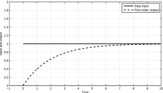10.

2.4.5 First order transfer function A first order transfer function is a fraction with one pole in its denominator which in the form of block diagram could be illustrated as shown in Figure 2.11. 1 Q% + 1. X(s). Y(s). Figure 2.11 First order transfer function 2.4.5.1 Step input An step input of a system could be shown as. x(t) = A , where A is constant number for 0<t, and thus its output would be k(%) = l(%) × C(%) = 4 × “4b = 4(“4b y. y. ). .. We could derive its output in s-domain by partial fractions where we have k(%) = 4 − “4b . y. y“. And the inverse Laplace transform of the output in the time domain for 0<t could be readily calculated as below •(.) = w − w2 3” , ‡. and if we draw it for A=1 and Q = 2 we will have Figure 2.12, the output of a first order system to step input 2 Step input First order output. 1.8 1.6. Input and output. 1.4 1.2 1 0.8 0.6 0.4 0.2 0 −1. 0. 1. 2. 3. 4. 5. 6. 7. 8. 9. Time. Figure 2.12 Output of the first order function for step input. 19. 10.

2.4.5.2 Impulse input Considering an impulse input to the first order element the function of input at time domain is δ(t) = lim δ5p (t) where 5p →8. δ5p (t) =. w. 0 < . < .8 ,. 0 g.ℎ2P}f%2, where A is constant number. So the transformed form of impulse function is X(s) = w. So the first order output to the impulse input is. k(%) = l(%) × C(%) = w ×. “4b. =. y. “4b. .. The inverse Laplace transform of this the output in time domain for 0<t is y(.) = “ Ae3” , ‡. Assuming the output for A=1 and Q = 2 we have. y(.) = e3z . ‡. Drawing this output as a function of time we have Figure 2.13. 2 Impulse input First order output. 1.8 1.6. Input and output. 1.4 1.2 1 0.8 0.6 0.4 0.2 0 −1. 0. 1. 2. 3. 4. 5. 6. 7. 8. 9. 10. Time. Figure 2.13 Output of the first order function for impulse input The output of the first order system to an impulse input shows the damping effect of first order element where the amplitude of the output signal starts from w⁄Q = 1⁄2 , and attenuate to zero at infinite by an exponential speed.. 20.

2.4.5.3 Ramp input The ramp input to the first order function could be shown as a line with slope of A for 0<t as below Œ(.) = w. where A is constant number. And thus its Laplace transform in s-domain would be l(%) =. And therefore we could find the output as. y. 4z. .. k(%) = l(%) × C(%) = 4z × “4b = 4z (“4b y. y. ). The output in time domain is calculated through finding partial fractions k(%) = w( z − + “4b ) “. 4. 4. “z. And using inverse Laplace transformation we could find output of the system in time domain for 0<t •(.) = w(. − Q + Q2 3” ) , ‡. and for A=1 and Q = 2 the output is. •(.) = (. − 2 + 22 3z ) , ‡. and if we draw it as a function of time we will have Figure 2.14. We observe that the first order system makes a steady state error equal to Q = 2 in response to the ramp input. 10 Ramp input First order response. 9 8. Input and output. 7 6 5 4 3 2 1 0. 0. 1. 2. 3. 4. 5 Time. 6. 7. 8. 9. Figure 2.14 Output of the first order function for ramp input. 21. 10.

2.4.6 Second order transfer function The second order transfer function has two poles or in the other word two zeros in its denominator which in the form of block diagram is shown in Figure 2.15. X(s). t. % +2. t%. Y(s). +. t. Figure 2.15 Second order transfer function. where t is natural frequency and damping ratio. The location of denominator’s zeros have a fundamental impact on the behavior of the system. The zeros could be derived by % + 2 The value of If 0 < If. =1. <1. t%. +. t. = 0 , and therefore we could find zeros as below. % , = − t ± t— − 1 . is important factor influencing on the shape of output and if % , = ±˜ t . %. ,. =−. %. If 1 <. t ,. ±˜. =−. t —1 t.. −. =0. .. % , = − t ± t — − 1. So we observe that by changing from zero to infinite the location of zeros changes on the complex plane as shown in Figure 2.16. And the response of the system changes by .. 0< 1<. ˜. <1. =0. 1<. ™. =1. =0 Figure 2.16 pole movement. 22.

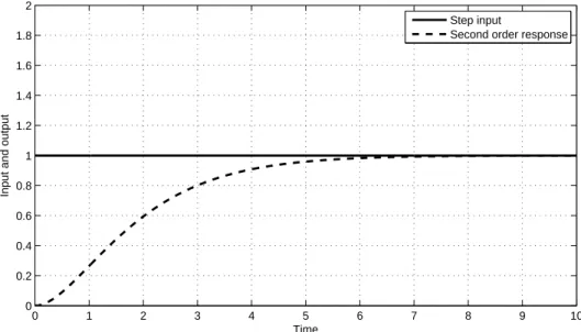
2.4.6.1 Step input The step input of the second order system alters by the value of damping ratio i.e., because it determines partial fractions and therefore the output of the system changes. Here we skip detail calculations and thus the outputs for different =0. and if 0 <. y(t) = 1 − cos. <1. •(.) = 1 −. =1. and if. › sœ•o‡ — 3ž z. sin(. t —1. t .,. −. . + cos3. •(.) = 1 − 2 3Ÿo 5 (1 +. and if 1 <. •(.) = 1 −. Ÿo. —ž z 3. (. › s†r ‡ 4r. values are as follow. So If. −. t .) › s†z ‡ 4z. ) ,. , ) ,. where % and % are two zeros of denominator. We could draw these outputs as function of time in Figures 2.17-20.. Figure 2.14 is for = 0 and t =1 and shows the response of the system is sinusoid without any damping. Figure 2.18 is for = 0.1 and t =1 and shows a sinusoid output which is damping over the time. Figure 2.19 is for = 1 and t =1 which is an exponentially increasing signal excluding any sinusoid signal. Figure 2.20 is for = 3 and t =1 which is another exponentially increasing signal having less damping compared with the = 1. 2 Step input Second order response. 1.8 1.6. Input and output. 1.4 1.2 1 0.8 0.6 0.4 0.2 0. 0. 1. 2. 3. 4. 5 Time. 6. 7. 8. 9. Figure 2.17 Output of the second order function for step input with. 23. 10. =0.

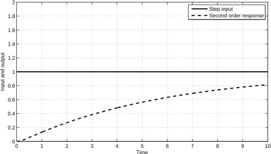
2 Step input Second order response. 1.8 1.6. Input and output. 1.4 1.2 1 0.8 0.6 0.4 0.2 0. 0. 1. 2. 3. 4. 5 Time. 6. 7. 8. 9. Figure 2.18 Output of the second order function for step input with. 10. = 0.1. 2 Step input Second order response. 1.8 1.6. Input and output. 1.4 1.2 1 0.8 0.6 0.4 0.2 0. 0. 1. 2. 3. 4. 5 Time. 6. 7. 8. 9. Figure 2.19 Output of the second order function for step input with. 24. 10. =1.

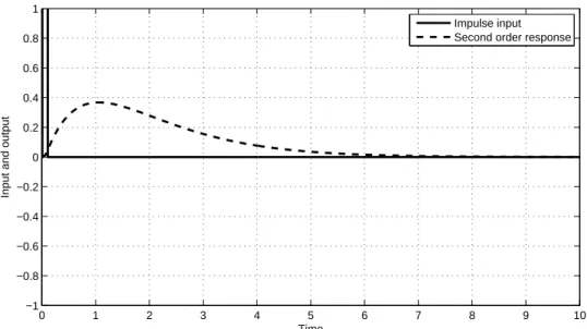
2 Step input Second order response. 1.8 1.6. Input and output. 1.4 1.2 1 0.8 0.6 0.4 0.2 0. 0. 1. 2. 3. 4. 5 Time. 6. 7. 8. 9. Figure 2.20 Output of the second order function for step input with. 10. =3. 2.4.6.2 Impulse input The impulse input of the second order system is also a function of damping ratio i.e., due to partial fractions. Changing partial fractions changes the output of the system in sdomain and as a result influence on the response of the system in time domain. Calculating the response of the system for different values of of the system in time domain. If = 0 and if 0 < and if. <1. =1. y(t) =. •(.) =. Ÿo. — 3ž z. t sin t —1. 2 3žŸo 5 sin. −. t —1. . ,. −. .. we could derive output. ,. •(.) = t .2 3Ÿo 5 . Drawing all of these equations as function of time we could derive the output of second. order system as follow.. Figure 2.21 is for = 0 and t =1 and shows the output of system to the impulse function which is sinusoid signal without any damping. Figure 2.22 is for = 0.1 and t =1 and shows a sinusoid response which is damping over time and its amplitude reduces to zero. Figure 2.23 is for = 1 and t =1 which is an exponential signal multiplying a ramp and has no sinusoid component. Figure 2.24 is for = 3 and t =1 which is another exponential signal but its amplitude is less than = 1 resulting more damping.. 25.

1 Impulse input Second order response. 0.8 0.6. Input and output. 0.4 0.2 0 −0.2 −0.4 −0.6 −0.8 −1. 0. 1. 2. 3. 4. 5 Time. 6. 7. 8. 9. 10. =0. Figure 2.21 Output of the second order function for impulse input with. 1 Impulse input Second order response. 0.8 0.6. Input and output. 0.4 0.2 0 −0.2 −0.4 −0.6 −0.8 −1. 0. 1. 2. 3. 4. 5 Time. 6. 7. 8. 9. Figure 2.22 Output of the second order function for impulse input with. 26. 10. = 0.1.

1 Impulse input Second order response. 0.8 0.6. Input and output. 0.4 0.2 0 −0.2 −0.4 −0.6 −0.8 −1. 0. 1. 2. 3. 4. 5 Time. 6. 7. 8. 9. Figure 2.23 Output of the second order function for impulse input with. 10. =1. 1 Impulse input Second order response. 0.8 0.6. Input and output. 0.4 0.2 0 −0.2 −0.4 −0.6 −0.8 −1. 0. 1. 2. 3. 4. 5 Time. 6. 7. 8. 9. Figure 2.24 Output of the second order function for impulse input with. 27. 10. =3.

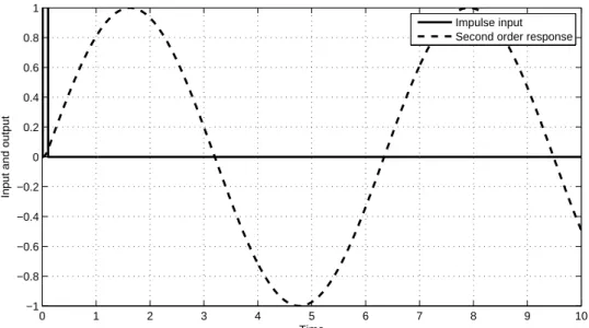
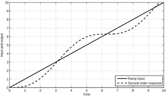
2.4.6.3 Ramp input The last input to the second order transfer function that we are going to analyze is the ramp input which is again a function of damping ratio i.e. . Having different damping ratio influence on the output of the system in both time and s-domains. The response of the system for ramp input and for different values of damping ratio is calculated as below. If. =0. and if 0 <. <1. =1. and if. •(.) = . +. •(.) = . − Ÿ + ž. o. Ÿo. Ÿo — 3ž z. sin(. t.. + ),. 2 3žŸo 5 sin(. t —1. •(.) = . − Ÿ − Ÿ 2 3Ÿo 5 sin( ž. o. Ÿo 5. o. −. . + ),. + 1).. These outputs could be drawn as a function of time to observe behavior of the system to ramp inputs in Figures 2.25-28.. = 0 and t =1 and shows the sinusoidal behavior of the output oscillating around a ramp signal without any damping. Figure 2.26 is for = 0.1 and =1 t =1 and shows a damping sinusoid output around ramp signal. Figure 2.27 is for Figure 2.25 is for. and t =1 which is a ramp signal without sinusoid component that finally produce a constant steady state error in the output. Figure 2.28 is for = 3 and t =1 which is another ramp signal causing more steady state error increasing over time. 10 9 8. Input and output. 7 6 5 4 3 2 Ramp input Second order response. 1 0. 0. 1. 2. 3. 4. 5 Time. 6. 7. 8. 9. Figure 2.25 Output of the second order function for ramp input with. 28. 10. =0.

10 9 8. Input and output. 7 6 5 4 3 2 Ramp input Second order response. 1 0. 0. 1. 2. 3. 4. 5 Time. 6. 7. 8. 9. Figure 2.26 Output of the second order function for ramp input with. 10. = 0.1. 10 9 8. Input and output. 7 6 5 4 3 2 Ramp input Second order response. 1 0. 0. 1. 2. 3. 4. 5 Time. 6. 7. 8. 9. Figure 2.27 Output of the second order function for ramp input with. 29. 10. =1.

10 9 8. Input and output. 7 6 5 4 3 2 Ramp input Second order response. 1 0. 0. 1. 2. 3. 4. 5 Time. 6. 7. 8. 9. Figure 2.28 Output of the second order function for ramp input with. 30. 10. =3.

2.5 Block diagram If the system is consist of only one component the analysis is easy but if the system includes different component with different inter-relationships we need to draw block diagram that shows the whole system with all of relationships among components. So that we could derive whole transfer function of the system for any desired outputs in response to any input. And therefore we could model a set of simultaneous differential equations representing a system. In this approach block diagram includes unidirectional, operational blocks representing transfer functions of the components of the system. (Dorf & Bishop, 2010, p.80). 2.5.1 Block diagram reduction A practical system may include many differential equations resulting in a complicated block diagram. And since analyzing such sophisticated block diagram might be complex, thus we need to reduce the block diagram to simple configuration. We could reduce a block diagram to a simpler version by a set of rules as shown in Figure 2.29. (cf. Dorf & Bishop, 2010 and Ogata, 2004) The first rule in Figure 2.29 shows multiplying two serial blocks and creating a single block which is multiplication of two transfer functions of two blocks, such that the input of whole system would be the input of first block and the output of whole system would be the output of second block. The second rule is Figure 2.29 represents the existence of feedforward in block diagrams. A feedforward takes the information from an upstream point of the system and feeding it forward in a point at downstream. If the position of branches are as shown in the second raw of the Figure then they will be combined to a single block. The third rule of Figure 2.29 is about a feedback path. A feedback path takes the information of the system at a downstream point and feed it back somewhere on the upstream of the block diagram. A system with a feedback path same as shown in the Figure 2.29 could be simply reduced to a single block. The forth rule of Figure 2.29 is about moving a summing point a head of a block diagram. But the difference is that the inverse of the block diagram of the first branch will be add to the second branch of the system. So that the input of second branch will be multiplied to the inverse of the block diagram of the first branch. The fifth rule of Figure 2.29 is opposite of the forth rule where the summing point moves behind the desired block. The effect of this movement is addition of the desired block diagram to both of the branches that enter to the summing point, so that the two inputs will be multiplied to the desired block diagram and then enter to the summing point.. 31.

Rule Transformation. Original. Equivalent. No.. block diagram. block diagram. 1. Combining serial blocks. 2. Removing the feedforward path. 3. Removing the feedback path. 4. Moving a summing point a head of block. 5. Moving a summing point behind of block. Figure 2.29 Block diagram reduction. 32.

2.5.2 Open and closed loop systems Block diagrams could be designed for the desired targets of the problem. There are two important types of block diagram: Open and closed loop diagrams. In the open loop diagram the control system do not take into account output of the system in the control policy (Golnaraghi & Kuo, 2010, p.7). The open loop means that the system output is not fed back to the upstream of the block diagram to be compared with the reference as shown in Figure 2.30 (Dorf & Bishop, 2010, p.2). Desired output Controller. Actuator. Process. Output. Figure 2.30 Open loop system On the other hand, a closed loop control system considers its output in the control policy and therefore the error between the actual and desired output will be reduced. A schematic representation of a simple closed loop system with only one feedback loop is shown in Figure 2.31. Desired output Error + −. Controller. Actuator. Process. Output. Sensor Figure 2.31 Closed loop system Comparing them we observe that in a closed loop system instead of desired output, the amount of error of desired output and actual output is the input of controller and indeed the error is reduced in this system. The feedback in a control system has a stabilizing role. The stability is a property of the system and shows how well a system could follow its input and a feedback loop can improve the stability but sometimes it is harmful for a stable system (Golnaraghi & Kuo, 2010, p.7). The open loop control system is missing part of information which is useful for accurate tracking of the input. A feedback loop could improve the performance of the system by using output information in the decision making process.. 33.

There is a general categorization of open loop system with and without taking into account the disturbances as shown in Figure 2.32 and 2.33, and closed loop systems as shown in Figure 2.34 and 2.35 (cf. Bubnicki, 2005) Disturbance. Desired output Controller. Actuator. Output. Process. Figure 2.32 Open loop system without taking into account disturbances Disturbance Desired output. Output Controller. Actuator. Process. Figure 2.33 Open loop system with taking into account disturbances Disturbance. Desired output +. Controller. −. Actuator. Output. Process. Sensor. Figure 2.34 Closed loop system without taking into account disturbances Disturbance Desired output. +. Output −. Controller. Actuator. Process. Sensor. Figure 2.35 Closed loop system with taking into account disturbances. 34.

2.6 Frequency response As mentioned before models might have different types of inputs which trigger systems and force them to produce the outputs. Among them sinusoidal function is an important input in the design and analysis of the systems. Frequency response is one of the most suitable ways to discover the response of a system with any order to a sinusoidal input. For instance electric demand follows an approximately sine curve. Figure 2.36 shows the demand of Tokyo bay area in summer peaks (Tepco illustrated, 2013). This sinusoid demand result in sinusoid pattern of LNG or other fuels in power plants.. Figure 2.36 Pattern of daily electricity usage Tokyo area (Source Tepco illustrated, 2013). 35.

Given the transfer function of a system as G(s), the function G(˜ ) is a complex function of frequency ω and can be shown as G(jω) = |C(˜ω)|∡C(˜ω) ,. where |C(˜ω)| and ∡C(˜ω) denote the amplitude and phase of C(˜ ) (Golnaraghi & Kuo, 2010, p26). This function shows the amplitude and phase of the response of the system at steady state condition and is used to derive Bode diagram of the system. The Bode diagram is the amplitude ratio and phase shift of the system compared with input for all frequencies from zero to infinity. Using the frequency response approach, transfer function of the system is described in the frequency domain with real C¢ (ω) = Re,C(˜ω)/, and imaginary parts. where we have and. C¤ (ω) = Im,C(˜ω)/,. |C(˜ω)| = —C¢ (ω) + C¤ (ω) , ∡C(˜ω) = tan3. ¥¦ (§) , ¥¨ (§). such that the amplitude and phase of the response is derived through the real and. imaginary parts of the C(˜ω) directly (Dorf & Bishop, 2010, p.557). Drawing the amplitude ratio and phase shift of the system compared with input, we could find frequency response of the system which is called Bode diagram as mentioned-above. And. since amplitude ratio and phase shift are both functions of frequency ω , we could find the frequency response by drawing them as a function of ω. The frequency response methodology is an appropriate technique that enables us to derive the performance of the system and its stability from above mentioned plots at the same time. We could find output. of the system for different test inputs with different frequencies, therefore in this methodology we could use measured data rather than a transfer function. Furthermore any system with any order could be analyzed and optimized by this method which can be done with transfer function analysis. Since we use frequency response in our study, we calculate Bode diagram of basic transfer functions in the following step. The bode diagram is 20 ©gA 8 |C(˜ )| and ∡C(˜ω), but we do not consider the log operator and only draw |C(˜ω)| in this research.. 36.

2.6.1 Gain Constant numbers are gains of the blocks or product of gains of multiple blocks. Since gains always appear in transfer functions and corresponding block diagrams we need to know what is the effect of a gain on the frequency response of the system. Assuming a gain with transfer function of we put s = jω in equation, thus The real part of the function is and the imaginary part is. G(s) = 2,. G(jω) = 2.. C¢ (ω) = 2, C¤ (ω) = 0.. So we have. |C(˜ω)| = √2 + 0 = 2,. and. ∡C(˜ω) = tan3. 8. = 0,. where amplitude ratio is 2 and phase shift is zero degree. We derive different result for negative gains, for instance substituting s = jω, we have The real part of the function is and the imaginary part is So we have and. G(s) = −5,. G(jω) = −5.. C¢ (ω) = −5, C¤ (ω) = 0.. |C(˜ω)| = —(−5) + 0 = 5, ∡C(˜ω) = tan3 (3 ) = 180. 8. Drawing bode diagram of G(s) = 2 and G(s) = −5 for different frequencies we derive Figure 2.37 and 2.38. Figure 2.37 shows that positive constant gain has same effect on the amplitude for frequencies without making any phase shift. But negative constant gain, although has same effect on the amplitude for all frequencies but decrease phase of the output by 180 degrees as shown in Figure 2.38.. 37.

Bode Diagram. Magnitude (abs). 10. 5. 0. −5. −10. Phase (deg). 180 90 0 −90 −180 1. 2. 3. 4. 5 Frequency (rad/s). 6. 7. 8. 9. 10. 8. 9. 10. Figure 2.37 Bode diagram of G(s) =2. Bode Diagram. Magnitude (abs). 10. 5. 0. −5. −10. Phase (deg). 180 90 0 −90 −180 1. 2. 3. 4. 5 Frequency (rad/s). 6. 7. Figure 2.38 Bode diagram of G(s) = -5. 38.