Aalto University School of Science
Degree Programme of Computer Science and Engineering
Matias Piispanen
Simulating timing and energy
consump-tion of accelerated processing
Master’s Thesis Espoo, May 11, 2014
Supervisor: Professor Heikki Saikkonen Instructor: D.Sc. Vesa Hirvisalo
Degree Programme of Computer Science and Engineering MASTER’S THESIS
Author: Matias Piispanen
Title:
Simulating timing and energy consumption of accelerated processing
Date: May 11, 2014 Pages: 73
Professorship: Software Technology Code: T-106
Supervisor: Professor Heikki Saikkonen
Instructor: D.Sc. Vesa Hirvisalo
As the increase in the sequential processing performance of general-purpose cen-tral processing units has slowed down dramatically, computer systems have been moving towards increasingly parallel and heterogeneous architectures. Modern graphics processing units have emerged as one of the first affordable platforms for data-parallel processing. Due to their closed nature, it has been difficult for software developers to observe the performance and energy efficiency character-istics of the execution of applications of graphics processing units.
In this thesis, we have explored different tools and methods for observing the execution of accelerated processing on graphics processing units. We have found that hardware vendors provide interfaces for observing the timing of events that occur on the host platform and aggregated performance metrics of execution on the graphics processing units to some extent. However, more fine-grained details of execution are currently available only by using graphics processing unit simulators.
As a proof-of-concept, we have studied a functional graphics processing unit sim-ulator as a tool for understanding the energy efficiency of accelerated processing. The presented energy estimation model and simulation method has been vali-dated against a face detection application. The difference between the estimated and measured dynamic energy consumption in this case was found to be 5.4%. Functional simulators appear to be accurate enough to be used for observing the energy efficiency of graphics processing unit accelerated processing in certain use-cases.
Keywords: GPU, CUDA, OpenCL, parallel processing, energy efficient computing, high performance embedded computing, GPU compute, GPGPU
Language: English
Aalto-yliopisto
Perustieteiden korkeakoulu Tietotekniikan tutkinto-ohjelma
DIPLOMITY ¨ON TIIVISTELM ¨A
Tekij¨a: Matias Piispanen
Ty¨on nimi:
Kiihdytetyn laskennan ajoituksen ja energiankulutuksen simulointi
P¨aiv¨ays: 11. toukokuuta 2014 Sivum¨a¨ar¨a: 73
Professuuri: Ohjelmistotekniikka Koodi: T-106
Valvoja: Professori Heikki Saikkonen
Ohjaaja: TkT Vesa Hirvisalo
Suorittimien sarjallisen suorituskyvyn kasvun hidastuessa tietokonej¨arjestelm¨at ovat siirtym¨ass¨a kohti rinnakkaislaskentaa ja heterogeenisia arkkitehtuureja. Mo-dernit grafiikkasuorittimet ovat yleistyneet ensimm¨aisin¨a huokeina alustoina yleisluonteisen kiihdytetyn datarinnakkaisen laskennan suorittamiseen. Grafiik-kasuorittimet ovat usein suljettuja alustoja, mink¨a takia ohjelmistokehitt¨ajien on vaikea havainnoida tarkempia yksityiskohtia suorituksesta liittyen laskennan suorituskykyyn ja energian kulutukseen.
T¨ass¨a ty¨oss¨a on tutkittu erilaisia ty¨okaluja ja tapoja tarkkailla ohjelmien kiih-dytetty¨a suoritusta grafiikkasuorittimilla. Laitevalmistajat tarjoavat joitakin ra-japintoja tapahtumien ajoituksen havainnointiin sek¨a is¨ant¨aalustalla ett¨a gra-fiikkasuorittimella. Laskennan tarkempaan havainnointiin on kuitenkin usein k¨aytett¨av¨a grafiikkasuoritinsimulaattoreita.
Ty¨on kokeellisessa osuudessa ty¨oss¨a on tutkittu funktionaalisten grafiikkasuori-tinsimulaattoreiden k¨aytt¨o¨a ty¨okaluna grafiikkasuorittimella kiihdytetyn lasken-nan energiantehokkuuden arvioinnissa. Ty¨oss¨a on malli grafiikkasuorittimen ener-gian kulutuksen arviontiin. Arvion validointiin on k¨aytetty kasvontunnistusso-vellusta. Mittauksissa arvioidun ja mitatun energian kulutuksen eroksi mitat-tiin 5.4%. Funktionaaliset simulaattorit ovat mittaustemme perusteella tietyiss¨a k¨aytt¨otarkoituksissa tarpeeksi tarkkoja grafiikkasuorittimella kiihdytetyn lasken-nan energiatehokkuuden arviointiin.
Asiasanat: GPU, CUDA, OpenCL, rinnakkaislaskenta, energiatehokas suorittaminen, korkean suorituskyvyn sulautettu laskenta, grafiikkasuoritinlaskenta, GPGPU
Kieli: Englanti
I would like to thank my instructor, Vesa Hirvisalo, for all the support and guidance during this thesis and the later stages of my studies. I am especially grateful for getting the opportunity to learn about different aspects of high-performance embedded computing beyond the offerings of regular university teaching. Additionally, I would like to thank Professor Heikki Saikkonen for finding the time to supervise my thesis.
I would also like to extend my thank you to all my colleagues at the department of Computer Science and Engineering at Aalto, especially the members of the Embedded Software Group for all the help and support I received during the thesis, and for all the coffee room discussions that were often entertaining and sometimes informative.
Finally, I would like to thank my parents for their patience, and for the overwhelming support I have received throughout my life.
Trondheim, May 11, 2014 Matias Piispanen
Abbreviations and Acronyms
API Application programming interface CISC Complex instruction set computing CPU Central processing unit
CTA Cooperative thread array
CUDA Compute unified device architecture DMA Direct memory access
DSP Digital signal processor
DVFS Dynamic voltage and frequency scaling FIFO First in, first out
FPGA Field-programmable gate array GPU Graphics processing unit
GPGPU General-purpose graphics processing unit computing HPEC High performance embedded computing
ioctl intout/ouput control ISA Instruction set architecture JIT Just-in-time
MIMD Multiple instruction, multiple data MISD Multiple instruction, single data OpenCL Open Computing Language RISC Reduced intruction set computing SIMD Single instruction, multiple data SIMT Singe instruction, multple thread SISD Single instruction, single data
Abbreviations and Acronyms 5
1 Introduction 9
2 Background 11
2.1 Parallel computing . . . 11
2.1.1 Trends in parallel computing . . . 11
2.1.2 Granularity of parallelism . . . 12 2.1.2.1 Instruction-level parallelism . . . 12 2.1.2.2 Task parallelism . . . 13 2.1.2.3 Data parallelism . . . 14 2.1.3 Flynn’s taxonomy . . . 14 2.1.4 Amdahl’s law . . . 15
2.1.5 Multithreading on symmetric multiprocessors . . . 15
2.1.6 SIMD computation . . . 16
2.2 Efficient accelerated processing . . . 17
2.2.1 Accelerators . . . 17
2.2.2 Energy efficient computing . . . 17
2.3 Execution timing . . . 18
2.3.1 Dynamic program analysis . . . 18
2.3.2 Simulators . . . 19
2.4 Linux device driver . . . 20
2.5 Energy consumption . . . 21
2.5.1 Power and energy . . . 21
2.5.2 Power consumption . . . 22
3 GPU computation environment 23 3.1 GPU accelerated processing . . . 23
3.1.1 Graphics processing unit architectures . . . 23
3.1.1.1 General graphics processing unit architecture 23 3.1.1.2 Mobile graphics processing units . . . 25
3.1.2 Parallel compute model on graphics processing units . 26 3.1.3 Programming models for GPU accelerated processing . 28
3.1.4 GPU execution context and scheduling . . . 29
3.2 Host platform for GPU accelerated processing . . . 29
3.2.1 Program compilation workflow . . . 29
3.2.2 Runtime library and GPU device driver . . . 31
3.2.2.1 GPU device driver and CUDA runtime library 31 3.2.2.2 Task scheduling . . . 32
3.3 Tracing of accelerated computing . . . 32
3.3.1 Tracing of host operations . . . 33
3.3.2 Tracing of operations on GPU . . . 33
3.3.3 Tracing with TAU Parallel Performance System . . . . 34
3.3.4 Profiling of GPU accelerated processing . . . 35
3.3.4.1 CUDA Profiling Tools Interface (CUPTI) . . 35
4 Measuring and simulating GPUs 36 4.1 Instrumentation . . . 36
4.1.1 Timing and energy model . . . 36
4.1.2 Instrumentation . . . 37
4.2 GPU Simulators . . . 38
4.2.1 GPU simulator structure . . . 38
4.2.2 GPU simulator survey . . . 39
4.2.2.1 Barra . . . 39
4.2.2.2 GPGPU-sim . . . 39
4.2.2.3 Multi2Sim . . . 39
4.2.2.4 GPU Ocelot . . . 40
4.3 Parallel GPU simulation framework . . . 40
4.3.1 Parallel simulation . . . 40
4.3.2 GPU accelerated many-core simulator . . . 41
4.3.3 Extending QEMU with a parallel simulator . . . 43
5 Benchmarks 46 5.1 Microbenchmarks . . . 46 5.2 Application benchmark . . . 47 5.2.1 Motivation . . . 47 5.2.2 Computer vision . . . 47 5.2.2.1 Software modifications . . . 48 6 Evaluation 50 6.1 Energy estimation method . . . 50
6.1.1 Power model . . . 50 7
6.1.1.3 GPU operating state modeling . . . 54 6.1.2 Measurement setup . . . 55 6.1.3 Trace analysis . . . 56 6.2 Results . . . 57 6.2.1 Microbenchmarks . . . 57 6.2.2 Face detection . . . 60
7 Simulating GPU energy consumption 62 7.1 GPU energy consumption observations . . . 62
7.2 Simulating GPU energy consumption . . . 63
7.3 Simulating future GPU architectures . . . 64
8 Summary 66
Chapter 1
Introduction
The time of continuous increase in the serial execution performance of pro-cessors has come to an end. It is no longer possibly to simply crank up the clock speeds of processors to gain more performance. We have reached the limits imposed by physical laws. It is increasingly more difficult to cool down modern high-end processors, which is why it is important to decrease their energy consumption. The problem chip manufacturers now face is not how to make faster processors but how to make more efficient ones.
The landscape of high-performance computing is inevitably changing. A clear paradigm shift is taking place from sequential processing towards par-allelism. The first step was the introduction of multi-core processors in the form on symmetric multiprocessing, but this approach has proven not to be scalable. While there are fields where domain specific many-core accelerators have already been used, it was not until recently when many-core processing truly hit the mainstream. This was made possible by the realisation that there already is a many-core accelerator present in most modern computers, the graphics processing unit (GPU).
The programming models available for graphics processing unit program-ming were understandably meant for the rendering of graphics. The first attempt to bring more general-purpose computing to GPUs was to map com-putation to graphical primitives and performing comcom-putation by essentially drawing the primitives on the screen. This was a very tedious and ineffec-tive way to perform computation, which led to more suitable programming models and languages, such as the CUDA and OpenCL standards.
The problem with developing GPU accelerated programs lies in the closed nature of GPUs. It is difficult to get meaningful feedback of the execution. Essentially GPUs are treated as a black box system that is given program code and data for execution and after a while you receive some sort of an output. Recently GPU vendors have improved the support for program
filing, but these tools and performance counters are meant for debugging system performance only. Especially in the field of embedded computing, programmers are often interested in other matters as well, such as the en-ergy efficiency of processing.
The focus of this thesis is exploring different tools and methods for ob-serving both the host platform and GPU execution. These tools make it possible to profile and instrument GPU accelerated programs to learn more about the timing and energy consumption of program execution. In many cases the only solution is to rely on simulation tools, which may even be desirable for developers as they may not have access to the real hardware they are developing for. We also present a power model that allows the esti-mation of energy consumption of GPU accelerated programs. The model is validated by comparing it against the energy consumption of real GPU hard-ware running a real-world application benchmark from the field of computer vision.
We will start off by describing the background information related to this thesis in Chapter 2 that consists mostly of basic concepts of parallel pro-cessing, computer architecture and energy consumption of electronics. In Chapter 3 we explain the current computation and programming models of desktop GPUs, as well as explain the structure of software components re-lated to GPU accelerated computing on the host platform, and present some program profiling tools and methods. Then, in Chapter 4 we explore the methods needed to instrument GPU execution, which is needed for the es-timation of the energy efficiency of execution. The instrumentation must be generally done by using simulators. The chapter focuses on presenting a number of GPU simulators with a different focus, including a state-of-the-art parallel GPU simulator that is being developed. In Chapter 5 we present the benchmarks needed for configuring and validating the power model pre-sented in Chapter 6. On top of the power model this chapter also presents the measurement setup and the obtained estimated and measured energy consumption results. Finally, in Chapter 7 we discuss the overall landscape of estimating energy consumption of GPU accelerated computing by means of simulation before wrapping up our finding in the summary in Chapter 8.
Chapter 2
Background
This section describes the general background of this thesis. The topics cov-ered in this chapter include basic concepts of parallel processing, computer architecture, simulation, and power and energy consumption of electronics. A well informed reader may skip this section. As a reference to the gen-eral concepts and problems of parallel computing you can use the report by Asanovic et al. [2006] on the landscape of parallel computing.
2.1
Parallel computing
2.1.1
Trends in parallel computing
For many years the increase in performance followed the so called Moore’s law [Moore, 1965] that states that the number of transistors on integrated circuits tends to increase by the factor of two approximately every two years. Many other characteristics of computers, such as capacities of hard drives, clock speeds of processors and even the overall computational performance, seemed to follow this trend for a long time. It is clear that this sort of exponential growth cannot continue forever due to the laws of physics. In his article ”The Free Lunch Is Over” Sutter [2005] famously declared that the time of growth of the serial processing performance of microprocessors is now over, which will force manufacturers and developers to focus on more parallel computing solutions. In case of mobile devices, the available battery power is the limiting factor that will likely force them towards multi-core, and eventually many-core, architectures [van Berkel, 2009].
The trend in recent years has been to increase the number of processing cores in processors instead of raising the clock speeds of processors. It seems that the four gigahertz clock frequency is becoming a glass wall that
stream processor manufacturers are not able to exceed without unorthodox cooling methods. Modern computers also usually contain other domain spe-cific processing elements such as graphics processing units and digital signal processors. As the amount of processing elements increases, so does the total potential computing power of computers.
The consensus seems to be that parallel processing will be come more important in the future. Research is already focusing on microprocessors that have hundreds, if not thousands, of low-power cores on the same chip. It is likely that as the price of manufacturing many-core chips decreases, the cores will become more and more specialized cores so that only parts of the chip are active at any given time. Current heterogeneity in systems is mostly limited to having different kinds of processing elements in the system.
2.1.2
Granularity of parallelism
There are many possible ways to achieve parallelism in computing. Paral-lelism can occur at different levels of granularity. Coarse-grained paralParal-lelism is usually more visible to the programmer than fine-grained parallelism. Dif-ferent types of parallelism are typically divided into classes of instruction-level parallelism, task parallelism and data parallelism.
2.1.2.1 Instruction-level parallelism
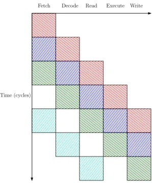
Execution on general purpose central processing units (CPU) at a high level of abstraction can be said to consist of three separate phases: instruction fetch, instruction decode and instruction execute. In practice these phases can be further split into multiple stages, such as memory operations, mathe-matical or logical operations, or other intermediate stages inside a processor. Each of these stages can take one or more clock cycles to execute. The typical length of an execution pipeline in current CPUs can range from two to even thirty stages. [Patterson and Hennessy, 2007, p. 370–374]
The stages in the execution pipeline are ordered and typically different stages use different functional units on the CPU. This makes it possible to have multiple instructions in execution simultaneously on the same processor as long as they are all in a different stage of execution and there are no dependencies between instructions. A new instruction can be issued every cycle as long as the instruction does not depend on the results of any of the instructions currently being executed. The pipeline length also affects how long it takes to fill a pipeline to reach maximum utilization. [Patterson and Hennessy, 2007, p. 370–374, 412–415]
CHAPTER 2. BACKGROUND 13
Time (cycles)
Decode
Fetch Read Execute Write
Figure 2.1: Example of pipelined execution. Squares of the same colour represent the execution of the same instruction.
Figure 2.1 shows an example of pipelined execution on a processor that has a five stage execution pipeline. The five stages are instruction fetch, in-struction decode, read memory, inin-struction execute and write-back to mem-ory. The x-axis represents time as clock cycles and y-axis represents the five pipeline stages. Boxes of the same colour represent the execution of a single instruction overtime. If a new instruction can be issued every clock cycle, a processor with five pipeline stages can be executing five different instructions at every given time. If new instructions cannot be issued due to for example data dependencies, it creates a so called bubble in the pipeline and maximum parallelism cannot be reached. In figure 2.1 the last instruction has to wait for one cycle before it can be issued for execution which creates a bubble in the pipeline.
2.1.2.2 Task parallelism
Splitting up a program so that different computational units execute differ-ent tasks is called task parallelism. Task parallelism is a more coarse-grained form of parallelism. It is the task of the programmer to write task parallel code by splitting the execution of the program into multiple processes or threads. An example of task parallelism would be dividing the work so that
one thread handles the rendering of graphics on the screen independently and in parallel to other threads in the process. Writing scalable task par-allel code is very challenging, especially in presence of communication and synchronization between threads. [Chapman et al., 2007, p. 192]
2.1.2.3 Data parallelism
Often there is a need to perform an identical operation for all the data items in a dataset. The difference to task parallelism is that the work partitioning is such that the sameoperation is performed concurrently and in parallel, but ondifferent data, instead of performing completely different tasks. [Chapman et al., 2007, p. 191–192] It is usually the responsibility of the programmer to partition the program execution for data parallelism, but under some circumstances a compiler can find opportunities for data parallelism and compile the program for parallel execution.
2.1.3
Flynn’s taxonomy
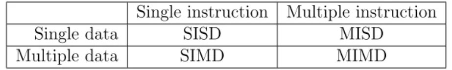
Flynn’s taxonomy [Flynn, 1972] is a traditional classification system for com-puter processor architectures. The taxonomy is used to classify processors into four categories on two axes, the amount of data being processed and the number of instruction streams being executed. The table of classifications is shown in figure 2.1.
Single instruction Multiple instruction Single data SISD MISD
Multiple data SIMD MIMD Table 2.1: Flynn’s taxonomy.
Flynn’s taxonomy classifies processors into following categories:
• Single instruction, single data (SISD) processors are typical se-quential processors. A single instruction stream is being executed that operates on a single set of data. Currently high-performance processors are moving towards more parallel architectures.
• Single instruction, multiple data (SIMD) processors execute a single instruction stream on multiple processing elements in lockstep, but each processing element operates on its own data. An example of SIMD processing is vector operations that are executed on special vector processing elements on processors. The SIMT execution model presented in 3.1.2 has a close relation to the SIMD model.
CHAPTER 2. BACKGROUND 15
• Multiple instruction, single data (MISD)processors execute mul-tiple instruction streams on separate processing elements, but they all operate on the same data. In reality there are very few consumer pro-cessors of this category. MISD architecture propro-cessors are generally used in systems that require high fault tolerance.
• Multiple instruction, multiple data (MIMD) processors execute multiple instruction streams on separate processing element and they all operate on their own data. This sort of execution is typically task parallel as described in section 2.1.2.2. [Wolf, 2007, p. 68]
2.1.4
Amdahl’s law
It is usually very difficult, if not impossible, to write completely parallel programs. In some cases parts of the program simply must be executed sequentially. For example, synchronization events may cause some threads to stall and wait for other threads to finish their task. The sequential parts of execution often dominates the overall execution time which results in often surprisingly bad overall performance. The guideline for finding the maximum expected improvement through parallelism is called Amdahl’s law. [Amdahl, 1967]
Amdahl’s law is presented in the formula Speed-up = 1
(1−P) + P N
, (2.1)
whereP is the proportion of the program that can be made parallel, (1−P) is the proportion of the program that is sequential and N is the number of processing elements available.
As an example, let’s observe the speed-up of a program where 75% of the program can be made parallel and it is processed on a four core processor. The expected maximum speed-up in such case given by Amdahl’s law is as follows: 1 (1− 3 4) + 3 4 4 = 2.286. (2.2)
The performance of such program can only be expected to double on a four core processor through parallelization.
2.1.5
Multithreading on symmetric multiprocessors
One of the most common ways for a programmer to achieve parallelism in an application is to write a multithreaded application. Multithreading refersto applications that consist of multiple instruction streams, called threads, that are executed concurrently and potentially in parallel. The creation and context switching of threads is much faster than those of processes, which is why they are preferred for concurrent computing. Parallelism can be achieved by executing threads on multiple processing elements. [Stallings, 2008, p. 161–165]
The most straightforward use for threads is to exploit task parallelism in applications [Wolf, 2007, p. 82]. In such programming model one task is usually assigned to one thread. Regular threads can also be used for data parallel computation. Data parallel computing models such as OpenMP follow a so called fork-join programming model, where the initial sequential thread creates a team of worker threads, or forks, and the parallel work is divided between the worker threads [Chapman et al., 2007]. When the parallel region ends, computation returns to the original sequential thread.
All threads belonging to the same process share the same resources. This introduces a need for synchronization between threads. Threads should not for example be allowed to write to the same location simultaneously. [Stallings, 2008, p. 166–167] The stalls in execution caused by synchro-nization essentially make processing sequential, which dramatically affects performance negatively, as stated by Amdahl’s law in section 2.1.4
2.1.6
SIMD computation
Many modern processors contain special hardware that can perform SIMD style vector operations. In SIMD computation, a single instruction performs an operation on multiple data items simultaneously. Vector operations are useful because many real-world applications contain computation that are prime candidates for SIMD computation. For example, most operations than manipulate pixel colour values are a good fit for SIMD computation, because pixel colours are typically represented as four separate 8-bit values (red, green, blue and alpha) and the same operation is applied to all four values. Special vector instructions are used for vector operations and it is often the programmers duty to explicitly declare vector operations in the code. [Wolf, 2007, p. 80–81]
CHAPTER 2. BACKGROUND 17
2.2
Efficient accelerated processing
2.2.1
Accelerators
Accelerators are computational units in computer systems that are designed to extend the functionality of the primary processor of the computer. Ac-celerators are designed to perform specific tasks, or at least specific types of tasks, more efficiently than the general-purpose host CPU. In the acceler-ated computing model, the host CPU offloads parts of the computation to accelerators. The motivation behind using accelerators is gaining either a considerable performance increase or reaching better energy efficiency.
Many different topologies are possible for accelerated systems. Accelera-tors may locate on the same chip as the primary processor or be on a separate chip attached to the CPU via a bus. Accelerators may either share memory with the primary processor or have their own memory.
Traditionally accelerators have been used to perform relatively simple fixed-function functionality. Examples of domains where accelerators have been widely used are accelerating complex mathematical operations, such as floating point arithmetic, signal processing and computer graphics. Recent trend has been to develop accelerators with more general-purpose computa-tional capabilities. Examples of such processors are modern graphics process-ing units, the Cell microprocessor and most recently Intel’s x86 many-core coprocessor Xeon Phi. The previously mentioned accelerators are mainly focused on exploiting data parallelism.
2.2.2
Energy efficient computing
For a long time, improving performance was the most important goal for commercial processor manufacturers. Since hitting the so called power wall, manufacturers have turned their focus on improving the efficiency of pro-cessors. Instead of plain performance, metrics of performance per watt and
performance per area have become increasingly important.
There are two different viewpoints to improving the efficiency of pro-cessors. Power consumption directly affects the amount of heat processors generate [Wolf, 2007, p. 21]. Heat generation is one of the biggest reasons for the rise of CPU clock speeds declining [Sutter, 2005]. Sequential perfor-mance can only be increased by improving the perforperfor-mance per watt ratio. On the other hand we can talk about energy efficiency when we want to stress the fact that embedded systems are often powered with batteries. Efficient computation increases the battery life of the whole system. [Wolf, 2007, p. 21]
Dynamic voltage and frequency scaling (DVFS) is a technique for lowering the power consumption of processors by scaling the clock speed and voltage of processors dynamically. There is a quadratic relationship between the energy consumption and operating voltage of a processor. In an ideal setting this would mean that by halving the clock speed and the operating voltage of a processor, you would get to one fourth of the original energy consumption. In practice there is a significant static component in the energy consumption of a processor that does not depend on the operating speed and voltage, which is often called leakage power. [Wolf, 2007, p. 86–87]
Simply adding more cores to CPUs feels intuitively like a good solution, but in practice it has been shown that this method does not scale well. Large portions of computer programs consist of sequential execution and writing completely parallel programs is difficult, if not impossible. Growing the number of cores also makes hardware design and memory management increasingly more difficult. A more realistic approach is to add more spe-cialized processing units on computers, such as the accelerators discussed in section 2.2.1. Specialized hardware is usually simpler in design, which lowers the energy consumption and often leads to better performance. Heteroge-neous computing, where parts of computation are offloaded to specialized processing units, tries to address the need for high performance and low energy computing. [Wolf, 2007, p. 267–275]
2.3
Execution timing
2.3.1
Dynamic program analysis
Dynamic program analysis means the analysis of programs by observing their execution either on a real processor or in a simulated environment. Program execution can be observed by either instrumenting the program by injecting code into the program that records desired information, or by explicitly mon-itoring the state of the real or virtual processor or memory during execution. There is usually a considerable amount of overhead associated with dynamic program analysis. The more often the state of execution is observed and logged, the bigger the overhead is.
Software profiling is a form of dynamic program analysis that aims to count the occurrences of different types of events, such as the number of times a function, basic block or instruction has been executed. Software profiling is typically used for optimizing program performance and identifying bottlenecks. [Ball and Larus, 1994]
CHAPTER 2. BACKGROUND 19
does not only count the number of different events, but records the sequence of events that have occurred during execution. Like with software profiling, execution tracing can be performed at different levels of granularity. A full execution timing model can be constructed by adding a timestamp to each event in the trace. [Ball and Larus, 1994]
2.3.2
Simulators
GPUs are much more closed systems compared to general-purpose CPUs. It is not possible to generate as thorough traces of programs that are being executed on the GPU. Vendors provide some tools that generate traces that allow developers to evaluate the performance of their applications. We are in-terested in building an estimated power model based on the execution traces, which requires more detailed tracing. Currently the only way to inspect the execution of GPU accelerated programs at the required level of detail is to use a GPU simulator.
The termsemulator and simulator are often used interchangeably. Both can be used to execute programs in place of an abstract or real machine. The difference between the terms lies in the model they are mimicking. The term emulator is used when the aim is to reproduce the behaviour of a real system. The term simulator is used when the system executes an abstract model. [Hirvisalo and Knuuttila, 2010, p. 2]
Simulators have numerous different use cases. Most commonly they are used to analyze the performance or the energy consumption of programs. Simulators can also be used to analyze the behaviour of processors before there is an actual physical processor available. Simulators can also be used for software debugging purposes. Simulation can be done by directly executing on the host processor and keeping track of the state of the guest processor, or by implementing an explicit simulator program that performs the execution and tracks the state of the guest processor. [Wolf, 2007, p. 126–130]
There is a clear trade-off between the speed of simulation and the accuracy with respect to the the characteristic of execution that is under analysis.
Functional simulators simulate the instruction set of a processor, but they do not model the microarchitecture of processors. A more accurate, but also much slower, simulator type is a so called cycle-accurate simulator. Cycle-accurate simulators model the state of the processor at microarchitecture level at the temporal granularity of a clock cycle. They also often keep track of processors resources, such as registers and memory, more accurately. The cost of cycle accuracy is a significant loss in performance. For accurate power modeling with simulation it is often necessary to also simulate other components of the computer, such as memory buses and memory. [Wolf,
2007, p. 131–132]
There are two basic methods for executing code in a simulator. Binary interpretation andbinary translation. Interpreting code in a simulator works much like a fetch-decode-execute loop in a real processor. This results in quite poor performance. A faster method is to translate the binary into the instruction set architecture (ISA) of the host processor either statically ahead of time or dynamically in blocks just-in-time (JIT) before the code is executed. While binary translation has a significant overhead, it is usually a much faster method compared to binary interpretation. [Hirvisalo and Knuuttila, 2010]
2.4
Linux device driver
Device drivers are computer programs that work as an interface between user programs and hardware. They provide a set of operations related to the hardware device they govern to user programs and manage the hardware resource so that it cannot be accessed in an illegal way. In Linux device drivers are typically implemented as a part of the kernel. User programs can invoke device services through a set of system calls. It is also the duty of the device driver to handle interrupts raised by the device.
Graphics processing units are typically character devices, meaning they are accessed as a stream of bytes like files. The typical system calls provided by a character device driver are open, close, read and write. Non-standard operations and hardware control operations are usually handled using the
ioctl (input/output control) system call. Devices can have a large set of operations that are accessed through the ioctl system call, and they are typically device specific operations. [Corbet et al., 2005, p. 1–7, 135–140] Typically user applications do not access device services directly through the system call interface, but they call functions of user-mode libraries that provide a higher level interface for applications.
Most hardware devices need to notify the kernel about certain events that have occurred on the device. Devices can interact with the kernel using
interrupts, that signal that there is an event that may require immediate attention. It is the duty of the device driver to implement functionality to handle interrupts raised by the hardware. There interrupt handlers are often split into kernel and user mode parts, often called the top and bottom halves. The kernel mode interrupt handler routine is run when an interrupt has been caught. The kernel mode interrupt handler routines should execute in a minimum possible amount of time because the execution blocks all other processes. What is actually required to be done in an interrupt handler
CHAPTER 2. BACKGROUND 21
depends on the nature of the interrupt. The handler should at least make sure the device can continue normal operation and that the interrupt will be handled appropriately. If the interrupt handling requires long computations, it can be split into one or more tasklets, that are user mode processes that will handle the computation. Tasklets are schedules like regular processes, so they do not interfere with regular execution of processes. [Corbet et al., 2005, p. 258–278]
2.5
Energy consumption
2.5.1
Power and energy
Energy and power are terms that in everyday speech are often used inter-changeably. Energy means the amount of work that a physical system is able to do on another system. The SI unit of energy is joule (J). In this thesis we are especially interested in the energy efficiency of computation, because en-ergy consumption has a direct effect of battery lifetime in embedded systems.
Power on the other hand is used to describe the rate of energy dissipation. The SI unit of Power is watt (W), which is joules per second. [Young et al., 2006]
We can describe the relationship between power and energy by defining
instantaneous power as follows: P = lim t→0 ∆E ∆t = δE δt . (2.3)
In this thesis we are interested in the electromagnetic energy dissipation of the computation of many-core processors such as GPUs. However, we cannot measure energy or power consumption directly. We can, however, measure the current (I) and voltage (V) of electronic circuits. Instantaneous power can be described as a function of voltage and current by using Ohm’s law andJoule’s first law, as defined in for example physics handbooks [Young et al., 2006]. Ohm’s law is defined as:
I = V
R. (2.4)
Joule’s first law is:
P =I2·R. (2.5)
By substitution, instantaneous power can be defined as a function of voltage and current at a given point in time t as follows, assuming a constant supply voltage:
P(t) = I(t)·V = V 2
R . (2.6)
Energy dissipation over a time interval T can be then defined through inte-gration: E = Z T 0 I(t)·V dt. (2.7)
2.5.2
Power consumption
The overall power consumption of a processor can be described with the following equation:
P ower =Dynamic power+Static power (2.8) Dynamic power is caused by the switching of transistors during execution of programs. As the name suggests, dynamic power consumption varies based on the nature of execution and the workload of the processor. Static power is the result of hardware architecture design and operating temperature, and it can be considered to be more or less constant, unless execution affects the operating temperature. [Hong and Kim, 2010]
Dynamic power in the above equation can be described to be proportional to the following formula:
P =ACV2f, (2.9)
where A is the activity factor, C is total capacitance, V is operating volt-age and f is the frequency of the clock. The above formula explains why power-saving techniques such as DVFS, described in Section 2.2.2, can yield significant energy savings. It if more efficient to ”race to idle” by complet-ing a task at a high peak frequency and then runncomplet-ing at a reduced clock frequency and operating voltage during idle states.
Chapter 3
GPU computation environment
In this chapter we present both the hardware and software platforms related to GPU accelerated processing. The GPU compute model differs quite dra-matically from typical program execution on CPUs. Section 3.1 presents the abstract hardware architecture of graphics processing units and the program-ming models for GPU accelerated processing. After that we take a look at the software stack on the host platform. Finally, we look at some methods on how it is currently possible to instrument and profile the execution of GPU accelerated programs.3.1
GPU accelerated processing
3.1.1
Graphics processing unit architectures
3.1.1.1 General graphics processing unit architecture
Graphics processing units are high throughput processors. Their processing power is achieved by having a large number of simple processing elements that perform computations in parallel. Originally graphics processing units were designed specifically for rendering of graphics, but as the graphics rendering pipeline became more programmable, the structure of GPUs became more suitable for general-purpose computing.
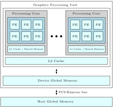
Figure 3.1 shows the high-level architecture of current desktop graphics processing units. A GPU consists of multiple processing cores. Typically the number of cores can vary from just a few up to a few dozen cores per GPU. The processing cores each execute their own stream of instructions. The actual computation is performed by the processing elements (PE) on the processing cores. Recent consumer GPUs have had up to 48 processing elements on each processing core. The trend on both mobile and desktop
L1 Cache / Shared Memory PE PE PE PE PE PE L2 Cache Processing Core
L1 Cache / Shared Memory
PE PE PE PE
PE PE
Processing Core
Device Global Memory
Host Global Memory Graphics Processing Unit
PCI-Express bus
Figure 3.1: High-level GPU architecture
GPUs has been to increase the total number of processing elements on the GPU to achieve higher throughput.
Current desktop GPUs contain a small cache, that can also be used as a programmable shared memory, on each processing core [NVIDIA, e, p. 10–11]. In the first generation GPUs that were used for general-purpose computation, only a smaller shared memory was available on the processing cores. The main method for hiding memory access latency is having a large number of threads ready to run and having a fast thread switching mechanism implemented in hardware. [Wang, 2010, p. VI-620] The current generation GPUs also have a larger L2 cache shared by all the processing cores for hiding global memory access latency.
Graphics processing units have a much larger number of registers com-pared to general-purpose processors. Each processing core typically has thou-sands of registers. The registers allocations are divided between a large num-ber of threads to avoid the need of context switches in the sense they are performed on CPUs. Having a fixed allocation of registers for each thread that is ready to be executed on a processing core simplifies the hardware needed for scheduling. [Kanter, 2009, p. 5–6]
Scheduling logic is located on the processing cores. Instructions are dis-patched to the core’s processing elements that execute the same instruction in parallel operating on their own data. This makes the execution
funda-CHAPTER 3. GPU COMPUTATION ENVIRONMENT 25
mentally SIMD-style computation as described in 2.1.6. [Kanter, 2009, p. 5–7]
Dispatch port
Operand collector
ALU FPU SFU
Result queue Processing Element
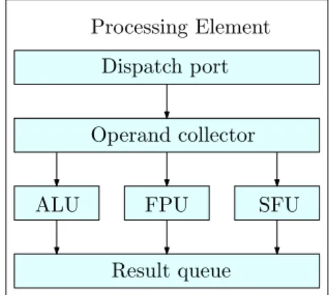
Figure 3.2: Abstract processing element architecture
Processing elements on the processing cores consist mostly of functional units. The number of different functional units may differ. GPUs that are fo-cused on graphics rendering performance typically have high single-precision floating point performance, while GPUs aimed for general-purpose computa-tion and scientific computing may have more double-precision floating point units. [Kanter, 2009, p. 5–7] GPUs capable of general-purpose computation also have integer arithmetic logic units and Special Function Units (SFU) that are responsible for performing special math operations such as square root, sine and cosine [Wong et al., 2010]. There may be other units on the processing element that aim to reduce memory operation latencies, such as the operand collector and result queue units in the example processing element structure presented in figure 3.2 [Kanter, 2009, p. 5–7].
3.1.1.2 Mobile graphics processing units
Graphics processing units on mobile devices such as mobile phones are very similar to desktop GPUs. They are expected to perform mostly similar tasks, although their performance is not on par with modern desktop GPUs. Mobile GPUs need to be extremely energy efficient, because they are powered by batteries and there is typically no active cooling elements such as fans cooling them down. [Akenine-Moller and Strom, 2008]
The high-level memory architecture of a typical mobile system on a chip (SoC) can be seen in figure 3.3. The biggest difference between mobile and desktop GPUs is that mobile GPUs are typically located on the same chip as the host CPU processor. The CPU and GPU also often share the system main
CPU GPU Accelerator HW L1 Cac he L2 Cac he Mobile Chip System RAM Flash memory
Figure 3.3: Memory architecture of a typical mobile chip. [Akenine-Moller and Strom, 2008]
memory which is located off the chip. Sharing memory eliminates the need for explicit memory transfers between CPU and CPU memories. Mobile devices usually have domain specific accelerators for multimedia operations, such as video encoding and decoding. The accelerators aim to improve performance and energy efficiency. [Akenine-Moller and Strom, 2008]
3.1.2
Parallel compute model on graphics processing
units
The parallel compute model on GPUs, originally called general-purpose graph-ics processing unit computing (GPGPU), is a data parallel computing model. A commonly used term for the execution model is single instruction, multi-ple thread (SIMT), which is a marketing term coined by NVIDIA. The slight difference compared to SIMD vector computing is that the threads in the SIMT model perform the computations on the data items of the given vector lane sequentially one by one as scalar operations. While the threads execute the same instructions simultaneously, each thread can still have their own logical control flow by masking out computations in divergent branches. The GPU compute model is close to the single program, multiple data (SPMD) model where data is partitioned for parallel execution on different proces-sors [Algorithms and of Computation Handbook, 1999].
In the current compute model it is the responsibility of the programmer to manage memory on the GPU and explicitly handle memory transfers between host and device memories. The input data needs to be transferred to the GPU before computation can be done, and the results usually must be transferred back to the host memory. A typical application that uses the GPU as an accelerator takes the following steps:
CHAPTER 3. GPU COMPUTATION ENVIRONMENT 27
• Copy data from host to device buffers.
• Launch compute kernel for computation on the GPU device.
• Copy results back from device to host buffers.
• Deallocate buffers. [Gaster et al., 2011, p. 16–26]
The parallel regions of code that can be efficiently executed on a GPU are typically loop nests that iterate over a large amount of data. These parallel regions are implemented as so called kernel functions. The kernels are offloaded to the GPU for execution using a large number of threads which are all executing the same kernel function. The only difference between the threads is that they all have a unique index number which is used to determine their control flow and the data the thread will be working on. [Gaster et al., 2011, p. 16–19]
In addition to specifying the number of threads that perform the com-putation, the programmer needs to explicitly divide the threads into blocks called cooperative thread arrays (CTA) or workgroups [Gaster et al., 2011, p. 17–19]. GPUs schedule threads of the same CTA for computation on the same processing core. The motivation behind dividing threads into blocks is to avoid context switches in the traditional sense during computation. As presented in section 3.1.1.1, GPUs hide memory access latency by having a large number of threads ready to run. When a CTA is scheduled for execu-tion on a processing core, registers and shared memory are allocated for all the threads in the CTA so that they are all potentially ready to be executed. On the other hand, the amount of threads in a CTA limits the amount of registers and memory that can be allocated to a single thread. Finding the optimal CTA size is an application specific problem.
Another reason for dividing threads into blocks explicitly is to achieve scalable computation. CTAs can be scheduled to any processing core for computation, because by definition the computation of one CTA must be able to be done independently of others. The block structure makes it possible to accelerate the execution efficiently on GPUs with a different number of processing cores. [Gaster et al., 2011, p. 17–19]
As the threads of the same CTA are executing on the same processing core, they also share the same memory local to the core. This also allows the threads belonging to the same CTA to synchronize. However, synchro-nization between threads in different blocks is possible only by exiting the kernel execution and returning to sequential host code for synchronization. [NVIDIA, e, p. 6]
A more fine-grained scheduling unit in the execution model is what NVIDIA calls a warp and AMD calls wavefront. A warp is a group of threads of the same CTA, in current compute model 32 threads, that are scheduled for exe-cution on a processing core in parallel. The threads in the same warp always execute the same instruction with their own data in lockstep. Branching is handled by masking out the computation of threads that are not taking the branch currently in execution. [Wong et al., 2010]
3.1.3
Programming models for GPU accelerated
pro-cessing
General-purpose computing on graphics processing units (GPGPU) emerged as an exploitation of vertex and pixel shader programs used for computer graphics. In the shader based GPGPU programming model, input data was represented as a texture and it was drawn into a scene on a plane facing the camera so that each pixel colour value on the view plane represented a data item in the input data array. Pixel shaders were written to sample the input data texture, perform computation and write the output to another texture that could be read back to the host. While it was possible to get noticeable speedups, the programmability of shader based GPGPU computation was really low.
The first programming model actually designed for general-purpose GPU accelerated processing to emerge was NVIDIAs CUDA (Compute Unified Device Architecture) [NVIDIA, a]. In CUDA, the kernel functions, described in section 3.1.2, are implemented using CUDA C or CUDA C++. CUDA C/C++ are subsets of C and C++ languages. Compared to shader program based programming, the programmability of CUDA programs is dramatically better. However, the kernel functions are still written using a relatively low level language. CUDA programs can only be executed on NVIDIA’s graphics processing units.
As a response to CUDA, an open framework called OpenCL [Khronos Group] was developed. OpenCL is governed by Khronos Group. OpenCL resembles the functionality of CUDA very closely. Kernel functions are writ-ten using OpenCL C, which is a subset of C99 language. The host side library also has a very similar interface. The biggest difference to CUDA is that OpenCL programs can be executed on GPUs of multiple vendors, CPUs, field-programmable gate arrays (FPGA) and other accelerator hardware.
Recently, other parallel processing programming models have also emerged. There is a growing need for a high-level programming model that would al-low widespread adoption of accelerated parallel processing. OpenACC
[Ope-CHAPTER 3. GPU COMPUTATION ENVIRONMENT 29
nACC] is one standard that aims to provide an easy and familiar program-ming model that would still reach performance that is comparable to lower level computation models. OpenACC uses a similar compiler directive based approach as OpenMP, an existing parallel processing framework aimed for shared-memory parallelism on CPUs.
On mobile devices there are currently at least two programming models that have expressed the intent of supporting parallel computation on mobile GPUs, OpenCL and Renderscript [Google] on the Android platform. There are already multiple OpenCL comformant mobile GPUs on the market. GPU compute support was included to Renderscript in Android version 4.2.
3.1.4
GPU execution context and scheduling
Computation is scheduled on GPUs hieracrhically with different levels of granularity. On the coarsest level the global scheduler schedules blocks of ker-nels for execution on the processing cores. Processing cores may be scheduled to execute blocks belonging to different kernels simultaneously on modern GPUs. [Kanter, 2009, p. 4] However, it is not possible to have kernels from different streams executing at the same time [Kato et al., 2012]. Executing multiple kernels simultaneously can improve utilization.
Finer grained scheduling is performed by the processing cores. The cores issue instructions from warps that are ready to run. GPUs do not perform context switching like traditional CPUs. They rely on having enough warps ready to run so that there are always instructions ready to be issued for execution.
Another big difference compared to traditional CPUs is that GPU compu-tation in current generation GPUs is non-preemptive. Once a compute kernel has been launched for computation, the GPU will keep processing the kernel until all threads belonging to the kernel launch have finished computation. [Kato et al., 2012]
3.2
Host platform for GPU accelerated
pro-cessing
3.2.1
Program compilation workflow
This section presents the compilation flow of NVIDIA’s LLVM based CUDA and OpenCL compiler called nvcc. Other vendors, such as AMD, may have different terminology and they may use different intermediate languages and compiler frameworks for compilation, and they ultimately target a different
ISA, but the overall structure of the workflow still mostly applies to them. This section considers NVIDIA’s implementation because most of the GPU simulators are based on the PTX intermediate language used by them. The compiler is open source as a part of the LLVM compiler project up to the PTX code generation phase. The final ISA code generation is performed by a closed source library.
.cu
CUDA front-end
LLVM optimizer
PTX code generation
PTX
PTXAS
CUBIN
n
vcc
Figure 3.4: Workflow of the nvcc compiler. [NVIDIA, f]
The nvcc compiler workflow for a CUDA application has multiple steps as shown in figure. Kernels written with CUDA C or OpenCL C are first separated from the host code by the language specific front end. The kernels are then translated to the NVVM intermediate representation. NVVM IR is based on the LLVM intermediate language. NVVM extends the LLVM IR with a set of rules and intrinsics related to the parallel compute model, but it is fully compatible with existing LLVM IR tools. Standard LLVM optimizer passes also work on the NNVM IR. [NVIDIA, f]
The last phase of the open source part of the nvcc compiler is the PTX intermediate language code generation phase. The PTX code is already gen-erated to match the targeted GPU architecture, which makes the generation of native ISA binaries easier. Final ISA code generation is performed by a separate proprietary host assembler PTXAS which can either compile the
CHAPTER 3. GPU COMPUTATION ENVIRONMENT 31
binary offline or just-in-time as a part of the CUDA runtime. PTX represen-tation is embedded with the binaries enabling JIT compilation. [NVIDIA, f]
Using a virtual ISA that is fairly close to the final ISA has some benefits. While the generated PTX code is optimized for the targeted hardware ar-chitecture, the PTX IR itself is machine independent. This makes the PTX representations backwards compatible and it can be used to generate binaries for different generations of hardware and even for hardware of different man-ufacturers. From the vendor’s point of view it gives other parties a virtual ISA to target without releasing the specifications of their hardware’s ISA.
3.2.2
Runtime library and GPU device driver
3.2.2.1 GPU device driver and CUDA runtime library
Currently the device drivers for the graphics processing units of major GPU manufacturers are closed source and little documentation related to their functionality and interfaces are provided. There has been some efforts to reverse engineer the NVIDIA device driver and to implement open source alternatives. The Nouveau [Nouveau] open source drivers are already widely used as alternative graphics drivers for NVIDIA’s proprietary binary drivers. pscnv [PathScale] is a project forked from the Nouveau project, developed by PathScale, that aims to provide an open source driver for graphics and GPGPU computing.
The NVIDIA GPU driver is split into user-mode and kernel parts [NVIDIA, b]. Communication between the user-mode module and the kernel module occurs using system calls. GPU drivers generally use a large number of dif-ferentioctl system calls to invoke different operations. The ioctl calls used by GPU device drivers are not documented, but the previously mentioned open source projects have backwards engineered some of them. In facts, there is nothing that stops user applications from sending ioctl calls directly to the kernel driver to invoke GPU operations [Kato et al., 2012].
NVIDIA’s GPU driver offers a low level interface called CUDA driver API for directly configuring the GPU and launching compute kernels. CUDA driver API is an alternative to the higher level API provided by the runtime library giving slightly finer grained control over the GPU. The runtime library is built on top of the driver API. [NVIDIA, b]
A higher level interface compared to the Driver API is provided by the CUDA runtime library. The CUDA runtime library allows programmers to perform the basic GPU operations described in 3.1.2 without having to initialize the GPU explicitly. The runtime also allows native bindings for
other programming languages. [NVIDIA, b]
3.2.2.2 Task scheduling
GPU operations, such as memory copy operations and compute kernel launch-ing, are issued to channels that are called command queues or streams. Cur-rent generation GPUs do not allow multiple channels to access the GPU simultaneously, but channels can coexist and the GPU can switch from one channel to another. Streams are essentially First In, First Out (FIFO) queues of operations. [Kato et al., 2012]
Memory transfer operations are performed as either synchronous or asyn-chronous DMA transfers. Typically data transfers are performed synasyn-chronously, because the results of the data transfer are often needed either on the GPU or CPU before further computation can be performed. Asynchronous mem-ory transfers can overlap compute operations on the GPU. [Kato et al., 2012] Compute kernels are usually launched to the GPU asynchronously.
Proper synchronization in current GPU accelerated computing can be performed only on the host CPU. An explicit synchronize call waits for all commands that have been sent to the GPU to finish. Alternatively synchro-nization can be performed by using events that are defined in both CUDA and OpenCL programming models. Compute kernels for example can be queued so that their computation will not start before a set of specified events have been received. Events can be dispatched at the start and end of operations. [Kato et al., 2012]
3.3
Tracing of accelerated computing
The host and the accelerator have a different view of the processing of an application. The host sees accelerated blocks of computation and memory transfers as a set of operations. The accelerator performing the computation has a more detailed view of the execution. If we want to follow the overall execution of an application, we need to be able to combine the host and device views.
For following the execution from the host’s point of view, we need to track the start and end times of operations. The timing of operations can be done using different methods. Operations can either be measured indirectly from the host’s point of view, or directly on the accelerator if hardware support for such measurements is implemented. Measurements made on different devices using different clocks must be synchronized.
CHAPTER 3. GPU COMPUTATION ENVIRONMENT 33
3.3.1
Tracing of host operations
Programs initiate accelerated compute operations by calling functions in the runtime libraries. Some of these operations, such as allocating buffers in host memory, take place on the host platform. The parameters of the function calls may also reveal details of operations that may not be observable on the accelerator device. Host events can be observed by library wrapping of the runtime API [Malony et al., 2011]. The library wrapper can then intercept function calls before calling the actual runtime library.
3.3.2
Tracing of operations on GPU
The operations we wish to observe on the accelerator are the start and end times of the computation of compute kernels and memory transfers between host and accelerator memories. It would be desirable to also track host CPU events related to the accelerator operations. For example, launching a compute kernel on the accelerator actually consists of multiple different function calls to the driver API [Malony et al., 2011].
There are different methods for observing the start and end times of CUDA and OpenCL compute kernels. Execution can be observed using the
synchronous, event or callback methods. Support in both hardware and software may limit which instrumentation methods can be used.
Synchronous method is the simplest way to instrument compute kernel ex-ecution. By launching computer kernels for execution in a blocking manner, the host can measure the execution time using its own clock. The synchro-nized method is inaccurate because there is a delay between launching a kernel and when the execution actually starts, and also between the end of execution and when the host’s synchronization point. [Malony et al., 2011]
Event method relies on the event feature that is specified in both the CUDA and OpenCL language specifications. In the event method special
event kernels are queued to execute immediately before and after the mea-sured compute kernel. The event kernels record the state of the accelerator, meaning the event method uses the device clock for measurement. The event method at least in theory gives a more accurate measurement of the compute kernel execution time. The measured timestamps need to be synchronized with the CPU clock to obtain full system timing information. The event method needs support from hardware, which means that especially older hardware cannot use events for instrumentation. [Malony et al., 2011]
Callback method is the most accurate method for instrumenting accel-erator operations. Callbacks are defined in the recent versions of both the CUDA and OpenCL specifications. Like with the event method, the callback
method requires support from hardware and the device driver. The accel-erator triggers callback functions on the host when certain types of events occur. For timing, the events are the start and end events of compute ker-nels, but callback functions can be used to gather and handle performance measurements of other types too. [Malony et al., 2011]
On NVIDIA’s GPU hardware, CUDA Performance Tool Interface (CUPTI) provides an API for event and callback based instrumentation. CUPTI can be used to also read GPU device counters containing different performance metrics. [Malony et al., 2011] In CUDA toolkit versions prior to version five, there was a limitation that compute kernels could not be executed concur-rently when instrumenting execution using CUPTI.
3.3.3
Tracing with TAU Parallel Performance System
TAU Parallel Performance System [Shende and Malony, 2006] is a profiling and tracing tool for parallel programs. It is capable of instrumenting pro-grams ranging from regular multi-threaded applications to distributed com-puting at different levels of granularity. The recent versions of TAU have also included the capability to instrument GPU accelerated CUDA and OpenCL applications.TAU implements heterogeneous computing instrumentation by wrapping CUDA and OpenCL libraries and dynamically preloading the wrapped li-braries [Malony et al., 2011]. TAU was recently updated to use CUPTI fo instrumentation, which makes it possible to instrument kernel execution using any of the three instrumentation methods described in section 3.3.2.
CHAPTER 3. GPU COMPUTATION ENVIRONMENT 35
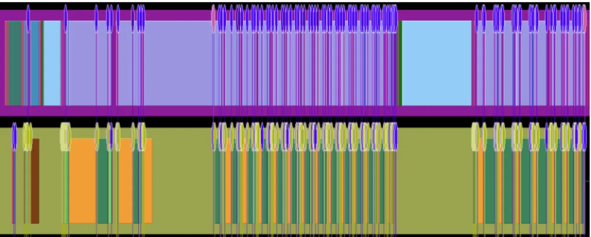
Figure 3.5 shows an example of a trace output from the TAU tool vi-sualised with the Jumpshot visualisation tool that is distributed with TAU. The application that was being traced was a modified face detection applica-tion using the OpenCV computer vision library. The applicaapplica-tion is presented in detail in Section 5.2.2. The coloured rectangles represent the execution of different functions over time. The upper row represents execution on the CPU and the lower row execution on the GPU. Keep in mind that execution of a function on the GPU in this context means a kernel launch of hundreds of threads executing the same function.
3.3.4
Profiling of GPU accelerated processing
3.3.4.1 CUDA Profiling Tools Interface (CUPTI)
CUDA Profiling Tools Interface (CUPTI) is a set of APIs that enable the creation of profiling and tracing tools, such as the TAU tool presented in the previous section. The four APIs provided by CUPTI are Activity API, Callback API, Event API and Metric API. Together they allow the tracing of calls to the CUDA runtime libraries, timing of the execution of CUDA kernels and collecting performance counter metrics of kernel execution.
The Metric API provides access to a set of metrics collected from actual execution of applications on a GPU. The set of reported metrics include metrics about number of instructions issued and executed, cache behaviour metrics and memory throughput metrics. The metrics are mostly suitable for evaluating the utilisation of the GPU. [NVIDIA, c]
Measuring and simulating GPUs
This section covers some methods that are currently available for observing the execution of GPU accelerated programs. We are especially interested in observing the timing and energy consumption of program execution. As GPUs are relatively closed systems, we have no choice but to use simulators to unveil details of the execution. At the end of this chapter we present a number of different parallel processing and GPU simulators that can be used to instrument parallel processing.4.1
Instrumentation
4.1.1
Timing and energy model
It is often not convenient, or even possible, to measure the energy consump-tion of a processor directly during execuconsump-tion. To overcome this observability issue, simulators are often used to trace the execution of a program. Ex-ecution traces can be used for building an abstract energy model for the system.
Power consumption consists of two parts: dynamic power and static power. Static power does not depend on the execution. It is a direct conse-quence of the chip design and operating temperature of the processor. Dy-namic power is the part that changes with runtime events of execution. Ba-sically each component that is activated on the processor consumes power. Static power, including power needed for the GPU memory, typically domi-nate the overall power consumption of a GPU. [Hong and Kim, 2010]
Accurate energy models are usually constructed using a cycle-accurate simulator that also simulates the memory and cache hierarchy. Such simula-tors are currently too slow to be used for software development purposes.
CHAPTER 4. MEASURING AND SIMULATING GPUS 37
cording to Miettinen and Hirvisalo [2009] the power consumption is roughly proportional to the cycle count of the processor. This makes it viable to use fast functional simulators for constructing approximate energy models if we can verify that the loss in accuracy is within acceptable bounds.
Different instructions take a varying time to execute and they consume different amount of energy. In practice we can group instructions into classes such as integer operations, floating point operations or memory load and store operations [Hirvisalo and Knuuttila, 2010]. For the energy model, we should count the amount of instructions belonging to each instruction class during execution. This can be done quite trivially during the execution loop in simulators. The power consumption of instruction classes can be calibrated through microbenchmarking which we will present in section 5.1.
Memory accesses have a significant impact on the overall power consump-tion. Simulating the full memory and cache hierarchies is fairly difficult and slow. Functional simulators often use abstractions of the memory hierarchy and simulate only a part of the cache hierarchy, if at all. For our purposes, it would be desirable to have at least the L1 cache simulated as there is a considerable difference between accessing L1 cache compared to other levels of the hierarchy.
Instruction counting is only applicable for estimating the power consump-tion of a single processor. For a many-core processor like a GPU, we must also keep track of where the computation takes place. Collange et al. [2009] have shown that the power consumption of a GPU rises piecewise linearly as the amount of active processing cores is increased.
4.1.2
Instrumentation
We wish to generate traces of the execution of kernels on GPUs. A trace is a record of a sequence of events that occurred during the execution of a program. We need to be able to count the number of executed instructions of different types and the number of different types of memory accesses.
The most common techniques for generating execution traces are instru-mentation and using simulators. Instruinstru-mentation generally means injecting code that emits events related to the execution. Simulators can generate executiong traces as they perform the execution of the program. For GPU accelerated programs, it is more convenient to generate traces of executed instructions by using a simulator.
It should be noted, that generating traces typically always slow down the execution of programs. Since the speed of execution even in a simulated environment is important to us, we should make sure that the overhead caused by tracing is as low as possible.
4.2
GPU Simulators
The motivation for using GPU simulators is that it is otherwise not possi-ble to trace the execution of GPU accelerated programs at a fine-grained level of detail. Profiling tools released by GPU vendors are only suitable for application performance analysis and tuning. In this section we cover the current state of state of the art GPU simulators. In section 4.2.1 we present the typical structure of popular GPU simulators and reasoning behind it. In section 4.2.2 we present some state of the art GPU simulators.
4.2.1
GPU simulator structure
There are two major hurdles GPU simulators need to overcome. The first fol-lows from the sheer number of processing units on graphics processing units. Simulating a many-core processor that has hundreds, if not thousands, of processing units on a multi-core processor with up to 6 physical cores with sufficient performance is intuitively a difficult problem to overcome. In real-ity simulators often work as sequential applications, which makes things even worse. The second problem is that the instruction set architecture of GPUs is not publicly available knowledge. While the ISAs have been partially backwards engineered, in practice simulators often work on the intermedi-ate language representations of programs instead of binaries. Emulating an intermediate language results in a loss in accuracy.
The simulators can be split into two different categories. Some simula-tors aim for purely functional simulation. Functional simulasimula-tors model the execution at instruction level. They do not keep track of the internal state of the simulated GPU. Functional simulators also usually do not simulate memory or cache behaviour. The other category is architectural simulators that try to model the internal state of GPUs at the granularity of a clock cycle. Architectural simulators also usually have at least L1 level cache sim-ulation and some sort of a device global memory simsim-ulation. Architectural simulators are usually aimed for timing and energy analysis and they can be an order of magnitude or more slower than functional simulators.
Most of the found simulators are aimed for analysing programs written with NVIDIA’s CUDA framework. Some of them also had support for the OpenCL standard. All the simulators included a software component that basically replaces the CUDA or OpenCL runtime library that intercepts the IO requests made by the application running on the host processor.
![Figure 3.3: Memory architecture of a typical mobile chip. [Akenine-Moller and Strom, 2008]](https://thumb-ap.123doks.com/thumbv2/123dok/2223079.2718943/26.892.252.640.195.328/figure-memory-architecture-typical-mobile-akenine-moller-strom.webp)
![Figure 3.4: Workflow of the nvcc compiler. [NVIDIA, f]](https://thumb-ap.123doks.com/thumbv2/123dok/2223079.2718943/30.892.302.617.339.724/figure-workflow-nvcc-compiler-nvidia-f.webp)