An economic order quantity model with pa

(1)

An economic order quantity model with partial backordering

and incremental discount

Ata Allah Taleizadeh

a

, Irena Stojkovska

b

, David W. Pentico

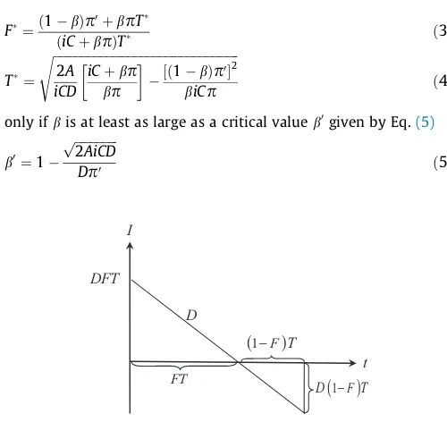
c,⇑ a_{School of Industrial Engineering, College of Engineering, University of Tehran, Tehran, Iran}

b_{Department of Mathematics, Faculty of Natural Sciences and Mathematics, Ss. Cyril and Methodius University, Skopje, Macedonia} c_{Palumbo-Donahue School of Business, Duquesne University, Pittsburgh, PA 15282, USA}

a r t i c l e

i n f o

Article history:

Received 14 August 2014

Received in revised form 2 December 2014 Accepted 5 January 2015

Available online 14 January 2015

Keywords:

EOQ

Incremental discounts Full backordering Partial backordering

a b s t r a c t

Determining an order quantity when quantity discounts are available is a major interest of material managers. A supplier offering quantity discounts is a common strategy to entice the buyers to purchase more. In this paper, EOQ models with incremental discounts and either full or partial backordering are developed for the first time. Numerical examples illustrate the proposed models and solution methods. Ó_{2015 Elsevier Ltd. All rights reserved.}

1. Introduction and literature review

SinceHarris (1913)first published the basic EOQ model, many

variations and extensions have been developed. In this paper we combine two of those extensions: partial backordering and incremental quantity discounts.

Montgomery, Bazaraa, and Keswani (1973) were the first to develop a model and solution procedure for the basic EOQ with partial backordering (EOQ–PBO) at a constant rate. Others taking somewhat different approaches have appeared since then,

includingPentico and Drake (2009), which will be one of the two

bases for our work here. In addition, many authors have developed models for the basis EOQ-PBO combined with other situational

characteristics, such asWee (1993) and Abad (2000), both of which

included a finite production rate and product deterioration,

Sharma and Sadiwala (1997), which included a finite production rate with yield losses and transportation and inspection costs,

San José, Sicilia, and García-Laguna (2005), which included models

with a non-constant backordering rate, andTaleizadeh, Wee, and

Sadjadi (2010), which included production and repair of a number of items on a single machine. Descriptions of all of these models

and others may be found inPentico and Drake (2011).

Enticing buyers to purchase more by offering either all-units or incremental quantity discounts is a common strategy. With the

all-units discount, purchasing a larger quantity results in a lower unit purchasing price for the entire lot, while incremental dis-counts only apply the lower unit price to units purchased above a specific quantity. So the all-units discount results in the same unit price for every item in the given lot, while the incremental dis-count can result in multiple unit prices for an item within the same

lot (Tersine, 1994). In the following we focus on the research using

only an incremental discount or both incremental and all-units

dis-counts together. SinceBenton and Park (1996)prepared an

exten-sive survey of the quantity discount literature until 1993, we will describe newer research, along with a short history of incremental discounts and older research which is more related to this paper.

The EOQ model with incremental discounts was first discussed byHadley and Whitin (1963).Tersine and Toelle (1985)presented an algorithm and a numerical example for the incremental dis-count and examined the methods for determining an optimal order

quantity under several types of discount schedules.Güder, Zydiak,

and Chaudhry (1994)proposed a heuristic algorithm to determine the order quantities for a multi-product problem with resource

limitations, given incremental discounts.Weng (1995)developed

different models to determine both all-units and incremental dis-count policies and investigated the effects of those policies with

increasing demand.Chung, Hum, and Kirca (1996)proposed two

coordinated replenishment dynamic lot-sizing problems with both

incremental and all-units discounts strategies.Lin and Kroll (1997)

extended a newsboy problem with both all-units and incremental discounts to maximize the expected profit subject to a constraint that the probability of achieving a target profit level is no less than

⇑ Corresponding author.

E-mail addresses:taleizadeh@ut.ac.ir(A.A. Taleizadeh),irenatra@pmf.ukim.mk, irena.stojkovska@gmail.com(I. Stojkovska),pentico@duq.edu(D.W. Pentico).

Contents lists available atScienceDirect

Computers & Industrial Engineering

(2)

a predefined risk level. Hu and Munson (2002) investigated a dynamic demand lot-sizing problem when product price schedules

offer incremental discounts.Hu, Munson, and Silver (2004)

contin-ued their previous work and modified the Silver-Meal heuristic algorithm for dynamic lot sizing under incremental discounts.

Rubin and Benton (2003) considered the purchasing decisions facing a buying firm which receives incrementally discounted price schedules for a group of items in the presence of budgets and space

limitations.Rieksts, Ventura, Herer, and Sun (2007) proposed a

serial inventory system with a constant demand rate and incre-mental quantity discounts. They showed that an optimal solution

is nested and follows a zero-inventory ordering policy.Haksever

and Moussourakis (2008)proposed a model and solution method to determine the ordering quantities for product multi-constraint inventory systems from suppliers who offer incremental

quantity discounts. Mendoza and Ventura (2008) incorporated

quantity discounts, both incremental and all-units, on the pur-chased units into an EOQ model with transportation costs.

Taleizadeh, Niaki, and Hosseini (2009) developed a constrained multi-product bi-objective single-period problem with

incremen-tal discounts and fully lost-sale shortages. Ebrahim, Razm, and

Haleh (2009) proposed a mathematical model for supplier selection and order lot sizing under a multiple-price discount environment in which different types of discounts including all-unit, incremental, and total business volume are considered.

Taleizadeh, Niaki, Aryanezhad, and Fallah-Tafti (2010)developed a multi-products multi-constraints inventory control problem with stochastic period length in which incremental discounts and

par-tial backordering situations are assumed.Munson and Hu (2010)

proposed procedures to determine the optimal order quantities and total purchasing and inventory costs when products have either all-units or incremental quantity discount price schedules.

Bai and Xu (2011)considered a multi-supplier economic lot-sizing problem in which the retailer replenishes his inventory from several suppliers who may offer either incremental or all-units

quantity discounts. Chen and Ho (2011) developed an analysis

method for the single-period (newsboy) inventory problem with

fuzzy demands and incremental discount.Taleizadeh, Barzinpour,

and Wee (2011)discussed a constrained newsboy problem with fuzzy demand, incremental discounts, and lost-sale shortages.

Taleizadeh, Niaki, and Nikousokhan (2011) developed a multi-constraint joint-replenishment EOQ model with uncertain unit cost and incremental discounts when shortages are not permitted.

Bera, Bhunia, and Maiti (2013)developed a two-storage inventory model for deteriorating items with variable demand and partial

backordering. Lee, Kang, Lai, and Hong (2013) developed an

integrated model for lot sizing and supplier selection and quantity discounts including both all units and incremental discounts.

Archetti, Bertazzi, and Speranza (2014) studied the economic lot-sizing problem with a modified all-unit discount transportation cost function and with incremental discount costs.

According to the above mentioned research, it is clear that no researchers have developed an EOQ model with partial

backorder-ing and incremental discounts. Taleizadeh and Pentico (2014)

developed an EOQ model with partial backordering and all-units discounts. In this paper we develop EOQ models with fully and par-tially backordered shortages when the supplier offers incremental discounts to the buyer.

2. Model development

In this section we model the defined problem under two differ-ent conditions: full backordering and partial backordering. But first we briefly discuss the EOQ model with full or partial backordering when discounts are not assumed. We use the following notation.

Parameters

A Fixed cost to place and receive an order

b The fraction of shortages that will be backordered

Cj The purchasing unit cost at thejth break point

D Demand quantity of product per period

g The goodwill loss for a unit of lost sales

i Holding cost rate per unit time

n Number of price breaks

qj Lower bound for the order quantity for pricej

P Selling price of an item

p

Backorder cost per unit per period

p

0

j The lost sale cost per unit at thejth break point of unit

purchasing cost,

p

0

j¼PCjþg>0 Decision variables

B The back ordered quantity

F The fraction of demand that will be filled from stock

Q The order quantity

T The length of an inventory cycle

Dependent variables

ATC Annual total cost

ATP Annual total profit

CTC Cyclic total cost

CTP Cyclic total profit

2.1. EOQ models with no discount

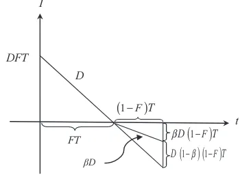
In this section we briefly discus EOQ models with fully or par-tially backordered shortages when discounts are not available. For the first case, the EOQ models with fully backordered shortages (seeFig. 1),Pentico and Drake (2009)derived the optimal values of

FandTas:

For the second case, the EOQ model with partial backordering,

Pentico and Drake (2009)showed that the values ofFandTthat minimize annual total cost are

F

(3)

2.2. EOQ model with incremental discount without shortages

Consider an EOQ model in which the supplier offers the

volume-based unit purchasing costs shown in Eq.(6)(Q_¼DT).

Cj¼

cost per order is:

Mj¼XjþCjDT; j¼1;2;. . .;n; ð7Þ

Then the purchasing cost per unit is (Tersine, 1994)

C0

and the optimal cycle length for ordering from the quantity from

thejth interval½qj;qjþ1Þis

The optimal order quantity isQ

j ¼DTj, with minimal annual total

The optimal order quantityQ

j is acceptable ifqj6Qj <qjþ1. If

Q

j <qj, then the optimal acceptable order quantity isQj ¼qj. If

Q

j Pqjþ1, then the optimal acceptable order quantity is

Q

j ¼qjþ1. For the latter two cases, the corresponding annual total

cost, calculated usingEq. (A1) in Appendix A, is the new optimal

annual total cost ATC

j. Finally, ATCj forj¼1;2;. . .;nare compared

to find the minimal value among ATC

j;j¼1;2;. . .;n, which will be the optimal annual cost for the EOQ model with incremental

dis-count, and the correspondingQ

j will be the optimal order quantity

for the EOQ model with incremental discount. This solution

proce-dure is justified, because we can prove that ifQ

j Pqjþ1, then there

is an order quantity which costs less to order thanQ

j does (see

Appendix A).

In the following sub-sections we model the defined problem under two different conditions: full backordering and partial

backordering, which are developed in Sections 2.3 and 2.4

respectively.

2.3. EOQ model with full backordering and incremental discounts

We will consider an EOQ model in which all shortages will be backordered and the supplier offers incremental volume-based

unit purchasing cost discounts. Then, according toFig. 1, the cyclic

total cost for ordering the quantity from the interval_½qj;qjþ1Þis

j is the purchasing cost per unit given by Formula (10).

Substituting Formula (10)into(13)and dividing byT we get the

annual total cost for ordering the quantity from the interval

½qj;qjþ1Þ:

Thus, the cost function that has to be minimized has the form

ATC_ðT;F_{Þ ¼}

The minimization is performed over the regionT>0;06F61 (see

Fig. 1).

Proposition 1. The functionATC_ðT;FÞ, defined by(14) and (15), is continuous.

Proof. SeeAppendix B.h

As a consequence ofProposition 1, the minimization problem

can be transformed into

min

Note that the sign < is changed into6in the upper bounds,

which is allowed by the continuity of ATC_ðT;FÞ. In what follows

we will use the notationTj andFjforTandF, respectively, when

we are minimizing the annual total cost for ordering the quantity

from the interval ½qj;qjþ1Þ defined by Eq.(14). To solve thejth

subproblem in(16), i.e. the problem

min

ðT;FÞ2Xj

ATCj_ðTj;FjÞ; ð17Þ

we first find the first partial derivatives of ATCjðTj;FjÞwith respect

toTjandFj.

Setting the first derivatives(18) and (19)equal to 0, and solving

the corresponding system with respect toTjandFj, remembering

thatTj>0, we get

To find the solution of the system(20) and (21), we substitute

(20) in (21), and obtain an equation with respect toFj:

iXjFjþD iC jFj

p

ð1FjÞTjðFjÞ ¼0; ð22Þ

which can be solved numerically with a solver like MatLab,

Mathematica, or Excel Solver. Let us denote the solution of (22)

(4)

by F

we have that there exists a solution F

j of (22) in the interval

[0, 1]. So, we can formulate the following proposition.

Proposition 2. There exists a solution F

j of Eq. (22), for which

06Fj 61.

Then, from Eq.(20)we have:

T

(17). The following proposition stands. Proving the global

optimal-ity ofðT

j;FjÞcan be also done as inStojkovska (2013).

Proposition 3. Assume that_ðT

j;FjÞ 2Xj, where Fj is the solution of (22), T

j is defined by (23), and Xj is the feasible region of

Subproblem (17). Then ðTj;FjÞ is the global optimal solution of

Subproblem(17).

Proof. SeeAppendix C.h

Note that wðFjÞ is a monotone nondecreasing function since

@w_ðFjÞ=@Fj¼@2/ðFjÞ=@F2j >0 (see (C6) in Appendix C). Thus the

solutionF

j of Eq.(22)is the unique solution in the interval [0, 1].

IfðT

global solution_ðT

j;FjÞof Subproblem(17)lies on the lower

bound-From the above discussion we can conclude that the global

optimal solutionðT_;_F_Þ_{that minimizes the annual total cost given}

in Eq. (15) is the pair _ðTj;FjÞ for which the corresponding

We have the following solution procedure for EOQ model with incremental discount and full backordering.

Solution procedure for the EOQ model with incremental discounts and full backordering

1. Forj= 1, 2,. . .,n:

1.1. Solve(22)using some numerical procedure, to obtainF

j.

2. Find the optimal solution as the pair _ðT

j;FjÞ for which the

corresponding ATCjðTj;FjÞis minimal over allj= 1, 2,. . .,n.

3. CalculateQ_¼_DT_and_B_¼_D_ð₁_F_Þ_T_.

2.4. The EOQ with incremental discounts and partial backordering

Unlike the full backordering model in which we minimized the annual total cost to obtain the optimal solutions, in the partial backordering model, in order to facilitate reaching the optimal

solution using the approach inPentico and Drake (2009), we will

first model the profit function and then by maximizing it we will

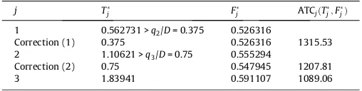
get the optimal solutions. According toFig. 2, in which it is clear

that the order quantity will beQ¼DT½Fþbð1FÞ, the unit

pur-whereXjis given by Eq.(8). Then the cyclic total profit for ordering

the quantity from the interval½qj;qjþ1Þis

Substituting (25)in (26)and dividing by Tgives the average

annual profit for ordering the quantity from the interval_½qj;qjþ1Þ:

After some algebraic transformations and letting

p

0

j¼PCjþg, we

(5)

ATP_ðT;FÞ ¼

Thus, the maximization problem can be written as

max

Note that the sign < is changed into6in the upper bounds for

the order quantity, which is allowed by the continuity of ATP_ðT;F_Þ

(seeAppendix D).

Since maximizing ATPjðT;FÞ is equivalent to minimizing the

function

Problem(30)is transformed into

max

Setting the first derivatives(33) and (34)equal to 0, and solving

the corresponding system with respect toTj andFj, remembering

thatTj>0, we have:

Substituting(35)into(36), we obtain an equation with respect to

Fj:

which can be solved numerically with a solver like MatLab,

Mathematica, or Excel Solver. Let us denote the solution of (37)

by F

is satisfied. Then, because of the continuity of the functionn_ðFjÞ, we

can formulate the following proposition.

Proposition 4. If Condition (38) is satisfied, then there exists a

solution F

Thus, if Condition(38)is satisfied,_ðT

j;FjÞis the solution of the

which is the optimal

cycle length for the cost ofCjin the EOQ model with incremental

discount without shortages (see Section2.2, Eq.(11)).

We can also prove that if Condition (38) is satisfied and

ðT

j;FjÞ 2X~j, then it is the global minimizer of the function

u

_j_ðTj;FjÞ over the domain X~j. The following proposition stands.

Proving the global optimality of ðT

j;FjÞcan be also done as in

Stojkovska (2013).

Proposition 5. Assume that Condition (38) is satisfied and ðT

j;FjÞ 2X~j, where Fj is the solution of(37), Tj is defined by (39),

and _X~_j is the feasible region defined by(30a). Then_ðT

j;FjÞ is the

global minimizer of the function

u

jðTj;FjÞover the domainX~j.

Proof. SeeAppendix E.h

As in the full backordering case, note thatn_ðFjÞis a monotone

non-decreasing function since @n_ðFjÞ=@Fj¼@2

g

ðFjÞ=@F2j >0 (see

(E6) in Appendix E). Thus, if Condition(38)is satisfied, the solution

F

j of Eq.(37) is the unique solution in the interval [0, 1], and if

ðT

j;FjÞ 2X~j, then ðTj;FjÞ is the unique global minimizer of the

function

u

jðTj;FjÞon the setX~j. If Condition(38)is not satisfied,

then 06b<b0j, which is equivalent to nð1Þ<0, and from nðFjÞ

being a monotonic function, we have that there is no solution of

Eq.(37) in the interval [0, 1]; consequently, partial backordering

cannot be optimal. So, in this case (06b<b0

j), the optimal decision

is either meeting all demand (EOQ model with incremental

discount and no shortages, Section2.2) with the optimal value of

the cycle lengthTj ¼

ffiffiffiffiffiffiffiffiffiffiffiffiffiffiffiffiffiffiffiffiffiffiffiffiffiffiffiffiffiffiffiffiffiffiffi

2_ðAþXjÞ=ðDiCjÞ

p

and the optimal value of

the fill rateF

j ¼1, or losing all sales withTj ¼ þ1andFj ¼0.

FromProposition 4and the above discussion about the values

forT

j andFj, we always haveTj>0 and 06Fj 61 when

Condi-tion (38) is met, but it might not be always true that

qj6DTjðFj þbð1FjÞÞ6qjþ1, in which case the pairðTj;FjÞwould

(6)

be infeasible and cannot be the minimizer of the function

u

_j_ðTj;FjÞ

on the setX~j. We have the following proposition.

Proposition 6. Assume that Condition (38) is satisfied, but ðT

j;FjÞ R X~j, where Fj is the solution of(37), Tj is defined by(39),

and X~j is the feasible region defined by(30a). Then the minimizer

ðT

j is the solution of

ðAþXjÞ

j is the solution of

ðAþXjÞ Proof. SeeAppendix F.h

Whenb<b0

jandb0jP0, as we saw earlier, the optimal decision

is meeting all demand from the EOQ model with incremental

dis-count and no shortages, i.e., the minimizer of

u

jðTj;FjÞlies on the

then the minimizer lies on the upper boundary T

j ¼qj1=D, and

the corresponding optimal profit isPDh_ðT

jÞ. Note that, in the

second case, we can exclude the point ðT

j;FjÞ from the set of

candidates for the optimal solution, since the corresponding order quantity is not the overall optimal order quantity (see

Appendix A).

When Condition (38) is met (bPb0j) and ðTj;FjÞ R X~j, but

neither(40a) or (40b)nor (41a) or (41b)is satisfied, this means

that partial backordering cannot be optimal, so the optimal decision is meeting all demand from the EOQ model with

incremental discount and no shortages (see Section2.2) or losing

all sales. In this case we should search for the optimal decision

as in theb<b0

jandb0jP0 case.

We can conclude that the global optimal solution_ðT_;_F

Þthat

maximizes the annual total profit, Function(29), is as one of the

points_ðT

j;FjÞfor which the corresponding profit is maximal over

allj= 1, 2,. . .,n.

The following solution procedure for the EOQ model with incre-mental discounts and partial backordering summarizes the details of the preceding theoretical results and their implications for the optimal solution.

Solution procedure for the EOQ model with incremental discounts and partial backordering

1. Forj¼1;2;. . .;n:

1.1. Calculateb0

jaccording to Formula(38).

1.2. IfbPb0_jP0 or b0_j<0, solve Eq. (37) to obtain F

j and

calculateT

j according to Formula(39).

1.2.1. If qj6DTjðFj þbð1FjÞÞ6qjþ1 (with q1¼0 and

jD, and take the higher profit. If the profit

from not stocking is higher, setT

j ¼ þ1andFj ¼0.

1.2.2. IfDT

jðFj þbð1FjÞÞ<qjandj2 f2;. . .;ng, then

(1.2.2.i) If one of the Conditions(40a) or (40b)is satisfied,

find F

(1.2.2.iii) Calculate the profit from not stocking,

p

0

jD, and set

T

j ¼ þ1andFj ¼0.

(1.2.2.iv) Compare the profits from (1.2.2i), (1.2.2.ii), (1.2.2.iii)

to determine the optimal (highest) profit if

DT

jðFj þbð1FjÞÞ<qj, and setTj ¼Tj andFj ¼Fj

for the optimal solution.

1.2.3. IfDT

jðFj þbð1FjÞÞ>qjþ1andj2 f1;. . .;n1g

(1.2.3.i) If one of the Conditions(41a) or (41b)is satisfied,

find F

(1.2.3.iii) Calculate the profit from not stocking,

p

0

jD, and set

T

(7)

(1.2.3.iv) Compare the profits from (1.2.3i), (1.2.3.ii), (1.2.3.iii)

to determine the optimal (highest) profit if

DT

by Formula(42). Compare the profit with the profit

from not stocking,

p

0

jD, and take the higher profit,

If the profit from not stocking is higher, set

T

given by Formula(42). Compare the profit with the

profit from not stocking,

p

0

jD, and take the higher

profit. If the profit from not stocking is higher, set

T

j ¼ þ1andFj ¼0.

2. Identify the maximum profit; the point_ðT

j;FjÞat which it is

attained is the global optimal solutionðT_;_F_Þ_.

3. If the optimal policy is partial backordering, calculate

Q_¼_DT_ð_F_þ_b_ð₁_F_ÞÞ _and _B_¼_b_D_ð₁_F_Þ_T_{. If the optimal}

policy is meeting all demand with incremental discount,

calcu-late Q¼DT_{. If the optimal policy is losing all sales, then}

Q¼0.

3. Numerical examples

We give numerical examples for both the full and partial back-ordering models with incremental discounts proposed in the above sections. The solution procedures are coded in Wolfram Mathem-atica, using built-in functions to solve nonlinear equations.

Example 1 (EOQ model with incremental discounts and full

backor-dering). We will use the values of all common parameters from the

numerical example for Taleizadeh and Pentico’s (2014)all-units

discount model: P= $9/unit, D= 200 units/period, i= 0.3/period,

p

= $2/unit/period, C¼ ðC1;C2;C3Þ= $(6, 5, 4)/unit, g= $2/unit,

q_{¼ ð}q₁;q₂;q₃_Þ= (0, 75, 150) units,

p

0_{¼ ð}

_p

0

1;

p

02;

p

03Þ= $(5, 6, 7)/unit.

We set the fixed order costA to $30/order. Values forT

j;Fj and

ATCjðTj;FjÞfor eachj¼1;2;3, are displayed inTable 1. Rows that

are noted as ‘‘correction (j)’’, display the values ofT

j andFj after

correctingT

j for not being in the intervalqj=D6Tj6qjþ1=D. Then,

ATCjðTj;FjÞis calculated for those corrected values forTj andFj.

According toTable 1, the annual total cost is minimized forj= 3,

so the overall optimal solution is T¼T₃¼1:83941; F¼

F

3¼0:591107, with the optimal costATCðT;FÞ ¼ATC3ðT3;F3Þ ¼

1089:06. The optimal order quantity isQ_¼_DT_¼₃₆₇_:_{881, with}

the maximum backordered quantityB_¼_D_ð₁_F_Þ_T_¼₁₅₀_:_424.

Example 2 (EOQ model with incremental discounts and partial

back-ordering). We use the same values for the parameters as in

Exam-ple 1, and we will vary the backordering parameter

b¼0:95;0:80;0:50. The results are displayed inTable 2. Rows that

are noted as ‘‘PBO correction (j)’’, display the values ofTj andFj

after correcting Q

j ¼DTjðFj þbð1FjÞÞ for not being into the

interval_½qj;qjþ1Þ, and if the correction is possible, i.e., if Conditions

(40a) or (40b)or Conditions(41a) or (41b)is satisfied. Then, ‘‘profit

(j)’’ is calculated for those corrected values forT

j andFj. If

correc-tions of the PBO model are done, then the row indicated with ‘‘NBO

model (j)’’ is filled, and ifQ

j ¼DTj from NBO model is not in the

interval½qj;qjþ1Þ, then the ‘‘NBO correction (j)’’ is done, and ‘‘profit

(j)’’ is calculated for those corrected values forT

j andFj. For each j,

the profit from not stocking is calculated and is displayed in the row ‘‘not stocking (j)’’. The highest profit is taken as the over-all profit.

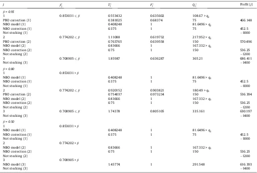
According to Table 2, when b¼0:95, the annual profit is

maximized for j= 3, under the partial backordering policy, with

T¼T₃¼1:85987 andF¼F₃¼0:636287, with the optimal profit

partial backordering policy, withT

¼T

3¼1:74378 andF¼F3¼

0:805105, with the optimal profit ATP_ðT_;_F_{Þ ¼}_ATP

3ðT3;F3Þ ¼

630:197. The optimal order quantity isQ

¼DT

ðF

þb_ð1F

ÞÞ ¼

335:161, and the maximum backordered quantity is

B_¼_b_D_ð₁_F_Þ_T_¼₅₄_:_3765.

Forb_¼0:50, the annual profit is maximized forj= 3, under the

policy of meeting all demand, withT

¼T

3¼1:45774;F¼F3¼1,

with the optimal profit ATP_ðT_;_F_{Þ ¼}₆₁₆_:_{393. The optimal order}

quantity isQ_¼_DT_¼₂₉₁_:_548.

All examples showed that if thejth optimal quantity is not in

thejth interval_½qj;qjþ1Þ, then it cannot be the overall optimal

quan-tity, even if it is corrected to the relevant interval endpoint. This was proved for the EOQ model with incremental discount and no

backordering (see Appendix A). It is left to be proven that this

might be also true for the proposed EOQ models with incremental discount – full and partial backordering respectively. From the examples we can see that keeping all parameters fixed and by varying the backordering rate, the total profit decreases when the backordering rate is decreasing.

4. Sensitivity analysis

There are at least two possible objectives for sensitivity analysis:

1. Assess the relative impact of mis-estimation of different model parameters on the model’s performance.

2. Assess the relative importance of the different model parame-ters in determining the values of the decision variables and the performance function.

4.1. Study plan

Both objectives can be addressed by changing a single parame-ter’s value by given percentages, repeating the analysis for each parameter of interest, using the same percentage changes.

Table 1

Results for EOQ model with full backordering and incremental discounts (Example 1).

j T

j Fj ATCjðTj;FjÞ

1 0.562731 >q2/D= 0.375 0.526316

Correction (1) 0.375 0.526316 1315.53

2 1.10621 >q3/D= 0.75 0.555294

Correction (2) 0.75 0.547945 1207.81

3 1.83941 0.591107 1089.06

(8)

The parameters in our model can be divided into two groups: (1) Parameters that have known values. (2) Parameters that are estimated. The second group can again be divided into at least two groups: those for which the estimates are probably fairly accu-rate and those that are less certain. For this model the breakdown is:

Less confident: backordering rate (b), goodwill loss for

stockout_ðgÞ, backordering cost (

p

)

There is one other relevant parameter group, the lost sale cost

per unit_ðf

p

0

jgÞ, but that is derived fromP, {Cj}, andg, so we do

not need to consider it separately.

We use the problem solved inExample 2withb= 0.80 as the

base case and then resolve it with changes of ±25%, ±20%, ±15%, ±10%, and ±5% in each of the estimated parameters, keeping all the other parameters constant. The performance measure is percent reduction in the average profit per period (ATP) for the variation relative to the optimal ATP from using the original parameter values.

Base case parameters:P= $9/unit,D= 200 units/period,A= $30/

order,i= 0.3/period,

p

= $2/unit/period,b¼0:80,C¼ ðC1;C2;C3Þ=

$(6,5,4)/unit, q¼ ðq1;q2;q3Þ= (0, 75, 150) units, g= $2/unit,

p

0¼

ð

p

0

1;

p

02;

p

03Þ= $(5, 6, 7)/unit.

Base case optimal values: T⁄_{= 1.74378,} _F⁄_{= 0.805105,}

Q⁄_{= 335.161,}_B⁄_{= 54.3765, ATP}⁄_{= 630.197/period.}

4.2. Study results

4.2.1. Effects of parameter changes on ATP

The details of the results of the changes in the estimated

param-eters are shown in Table 3. The percentage changes in ATP are

shown graphically inFig. 3. From these results we can draw the

following conclusions about how the estimated parameter changes affected the ATP:

1. As would be expected, the further the changed parameter’s value is from the value in the base case, the greater the decrease in the value of the ATP. There is one exception to this

conclu-sion,b, for which the percentage changes in ATP are identical

for changes inbof15%,20%, and25%. The reason for this

is that changes inbby these percentages bringbbelow its

crit-ical value for which partial backordering is optimal. As can be

seen in those rows ofTable 3, the optimal values of T andF

for those cases are 1.45774 and 1.0, giving Q= 291.548, and

B= 0. That is, the optimal solution for those cases is to use the

basic EOQ with no stockouts for these parameter sets. As shown inExample 2, the minimum value ofbfor which partial

backor-dering is optimal whenj= 3 is 0.708905, a reduction of 11.39

percent from the base case value of 0.80. Note also that an

increase of 25% in the value ofbincreases its value to 1.0, which

means that all shortages will be backordered. This solution,

which is shown in the last row of thebsection ofTable 3, results

in a decrease in ATP of over 3.5 percent.

2. For all parameters exceptbandg, decreases in the parameter

value resulted in greater reductions from the base case value than did the same-sized increases. The reason for this difference

Table 2

Results for EOQ model with partial backordering and incremental discounts (Example 2).

j b0

j Tj Fj Qj Profit (j)

b= 0.95

1 0.8530316b 0.553432 0.635602 108.67 >q2

PBO correction (1) 0.381025 0.68374 75 466.148

NBO model (1) 0.408248 1 81.6496 >q2

NBO correction (1) 0.375 1 75 452.5

Not stocking (1) 1000

2 0.7742026b 1.11088 0.619732 217.952 >q3

PBO correction (2) 0.763765 0.639558 150 570.496

NBO model (2) 0.83666 1 167.332 >q3

NBO correction (2) 0.75 1 150 536.25

3 0.7089056b 1.85987 0.636287 365.21 686.411

b= 0.80

1 0.853031 >b

NBO model (1) 0.408248 1 81.6496 >q2

NBO correction (1) 0.375 1 75 452.5

2 0.7742026b 0.920152 0.903821 180.49 >q3

PBO correction (2) 0.754037 0.973234 150 536.394

NBO model (2) 0.83666 1 167.332 >q3

NBO correction (2) 0.75 1 150 536.25

3 0.7089056b 1.74378 0.805105 335.161 630.197

b= 0.50

1 0.853031 >b

NBO model (1) 0.408248 1 81.6496 >q2

NBO correction (1) 0.375 1 75 452.5

2 0.774202 >b

NBO model (2) 0.83666 1 167.332 >q3

NBO correction (2) 0.75 1 150 536.25

3 0.708905 >b

NBO model (3) 1.45774 1 291.548 616.393

(9)

forbwas just discussed. The reason forgis unclear, but we note that the reductions in ATP for the same-sized negative and posi-tive changes are very close and less than 0.04 percent.

3. Changes inAresult in the least reduction in ATP, followed byg,

p

,D;i, andb, in that order. Note, however, that, with the

excep-tion ofband negative changes ini, the reductions in ATP are

less than one percent from the base case, even for 25 percent changes in the parameter value.

Since changes in the value ofbin 5 percent decrements, which

means changes of 4 percentage points, quickly resulted in solutions that did not use partial backordering, we looked at the effects of

changes in 1b, the complementary percentage of unfilled

demands that willnotbe backordered.b= 0.80 for the base case,

so the base case value of 1bis 0.20. Five percent changes in

1bare only one percentage point, which is much smaller than

the changes inb, so we looked at the effect of 10 percent changes

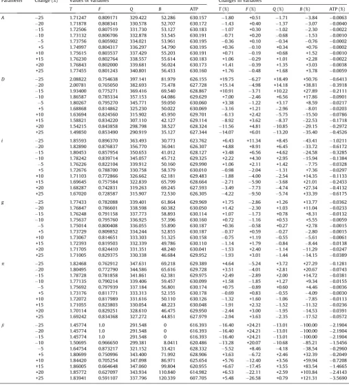
Table 3

Sensitivity analysis forExample 2problem withb= 0.80.

Parameter Change (%) Values of variables Changes in variables

T F Q B ATP T(%) F(%) Q(%) B(%) ATP (%)

A 25 1.71247 0.809171 329.422 52.286 630.157 1.80 +0.51 1.71 3.84 0.0063

20 1.71878 0.808341 330.578 52.707 630.172 1.43 +0.40 1.37 3.07 0.0040

15 1.72506 0.807519 331.730 53.127 630.183 1.07 +0.30 1.02 2.30 0.0022

10 1.73132 0.806706 332.878 53.545 630.191 0.71 +0.20 0.68 1.53 0.0010

5 1.73756 0.805902 334.021 53.961 630.195 0.36 +0.10 0.34 0.76 0.0002

+5 1.74997 0.804317 336.297 54.790 630.195 +0.36 0.10 +0.34 +0.76 0.0002

+10 1.75615 0.803537 337.429 55.203 630.191 +0.71 0.19 +0.68 +1.52 0.0010

+15 1.76230 0.802764 338.557 55.614 630.183 +1.06 0.29 +1.01 +2.28 0.0022

+20 1.76843 0.802000 339.681 56.024 630.173 +1.41 0.39 +1.35 +3.03 0.0038

+25 1.77455 0.801243 340.801 56.433 630.160 +1.76 0.48 +1.68 +3.78 0.0059

D 25 2.08822 0.754638 397.141 81.979 626.155 +19.75 6.27 +18.49 +50.76 0.6413

20 2.00781 0.765050 382.693 75.478 627.728 +15.14 4.98 +14.18 +38.81 0.3918

15 1.93400 0.775271 369.416 69.540 628.867 +10.91 3.71 +10.22 +27.89 0.2111

10 1.86587 0.785334 357.153 64.086 629.629 +7.00 2.46 +6.56 +17.86 0.0901

5 1.80267 0.795270 345.771 59.050 630.060 +3.38 1.22 +3.17 +8.59 0.0217

+5 1.68868 0.814862 325.230 50.022 630.069 3.16 +1.21 2.96 8.01 0.0203

+10 1.63694 0.824560 315.902 45.950 629.701 6.13 +2.42 5.75 15.50 0.0786

+15 1.58821 0.834220 307.110 42.127 629.114 8.92 +3.62 8.37 22.53 0.1718

+20 1.54215 0.843858 298.798 38.527 628.324 11.56 +4.81 10.85 29.15 0.2972

+25 1.49850 0.853490 290.919 35.127 627.344 14.07 +6.01 13.20 35.40 0.4526

i 25 1.85593 0.896370 363.493 30.773 623.762 +6.43 +11.34 +8.45 43.41 1.0211

20 1.82890 0.876837 356.770 36.041 626.307 +4.88 +8.91 +6.45 33.72 0.6172

15 1.80453 0.857954 350.653 41.012 628.127 +3.48 +6.56 +4.62 24.58 0.3285

10 1.78242 0.839714 345.057 45.712 629.325 +2.22 +4.30 +2.95 15.94 0.1384

5 1.76226 0.822104 339.912 50.160 629.990 +1.06 +2.11 +1.42 7.75 0.0328

+5 1.72676 0.788700 330.758 58.379 630.010 0.98 2.04 1.31 +7.36 0.0297

+10 1.71103 0.772866 326.662 62.181 629.483 1.88 4.00 2.54 +14.35 0.1133

+15 1.69645 0.757584 322.839 65.799 628.664 2.71 5.90 3.68 +21.01 0.2433

+20 1.68287 0.742831 319.263 69.245 627.593 3.49 7.73 4.74 +27.34 0.4132

+25 1.67020 0.728587 315.907 72.530 626.305 4.22 9.50 5.74 +33.39 0.6175

g 25 1.77433 0.782088 339.401 61.864 629.969 +1.75 2.86 +1.26 +13.77 0.0362

20 1.76847 0.786601 338.598 60.382 630.050 +1.42 2.30 +1.03 +11.04 0.0233

15 1.76248 0.791158 337.773 58.893 630.114 +1.07 1.73 +0.78 +8.31 0.0132

10 1.75637 0.795760 336.925 57.396 630.160 +0.72 1.16 +0.53 +5.55 0.0059

5 1.75014 0.800408 336.055 55.890 630.187 +0.36 0.58 +0.27 +2.78 0.0015

+5 1.73729 0.809852 334.244 52.855 630.187 0.37 +0.59 0.27 2.80 0.0015

+10 1.73067 0.814651 333.303 51.325 630.158 0.75 +1.19 0.55 5.61 0.0061

+15 1.72393 0.819503 332.339 49.786 630.110 1.14 +1.79 0.84 8.44 0.0138

+20 1.71705 0.824410 331.351 48.240 630.041 1.53 +2.40 1.14 11.29 0.0247

+25 1.71005 0.829375 330.338 46.684 629.952 1.93 +3.01 1.44 14.15 0.0389

p 25 1.82468 0.762912 347.631 69.218 629.389 +4.64 5.24 +3.72 +27.29 0.1281

20 1.80495 0.772790 344.586 65.616 629.728 +3.51 4.01 +2.81 +20.67 0.0743

15 1.78728 0.781858 341.861 62.381 629.975 +2.49 2.89 +2.00 +14.72 0.0381

10 1.77135 0.790214 339.406 59.457 630.099 +1.58 1.85 +1.27 +9.34 0.0155

5 1.75692 0.797939 337.184 56.801 630.174 +0.75 0.89 +0.60 +4.46 0.0036

+5 1.73176 0.811771 333.313 52.155 630.178 0.69 +0.83 0.55 4.09 0.0030

+10 1.72072 0.817989 331.616 50.110 630.126 1.32 +1.60 1.06 7.85 0.0113

+15 1.71055 0.823803 330.054 48.223 630.048 1.91 +2.32 1.52 11.32 0.0236

+20 1.70114 0.829251 328.610 46.475 629.950 2.44 +3.00 1.95 14.53 0.0391

+25 1.69242 0.834368 327.272 44.851 627.979 2.94 +3.63 2.35 17.52 0.0572

b 25 1.45774 1.0 291.548 0 616.393 16.40 +24.21 13.01 100.00 2.1904

20 1.45774 1.0 291.548 0 616.393 16.40 +24.21 13.01 100.00 2.1904

15 1.45774 1.0 291.548 0 616.393 16.40 +24.21 13.01 100.00 2.1904

10 1.50695 0.966650 299.381 8.0411 620.486 13.28 +20.07 10.68 85.21 1.5456

5 1.64754 0.873217 321.152 33.421 628.332 5.52 +8.46 4.18 38.54 0.2960

+5 1.80699 0.750996 343.400 71.992 628.906 +3.63 6.72 +2.46 +32.39 0.2049

+10 1.84420 0.705254 347.098 86.971 625.654 +5.76 12.40 +3.56 +59.94 0.7208

+15 1.86005 0.664648 347.060 99.804 620.955 +6.67 17.45 +3.55 +83.54 1.4665

+20 1.85772 0.627097 343.934 110.840 614.982 +6.53 22.11 +2.59 +103.84 2.4143

+25 1.83941 0.591107 337.796 120.339 607.705 +5.48 26.58 +0.79 +121.31 3.5690

(10)

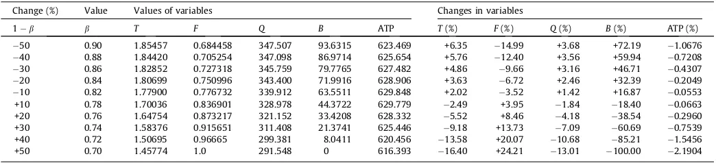
(2 percentage points each). As shown inTable 4andFig. 4, only a

50% increase in 1bto 0.30 orb= 0.70, resulted in the solution

to the problem with a changed value of 1bnot being partial

backordering. Sinceb= 0.70 is less than the minimum value ofb

for which partial backordering is optimal, this large an increase

in 1bresults in the optimal solution for the altered case to be

the EOQ with no stockouts (F= 1.0).

4.2.2. Effects of parameter changes on decision variable values

The percentage changes in the values of the four decision vari-ables that resulted from changing the parameter values are also

shown in Tables 3 and 4. As was the case with the percentage

changes in ATP, there are similarities and differences among the variables.

1. For all the parameters exceptb, the changes in T;F;Q, and B

were consistent as the parameter value increased from25%

to +25%. However, these changes were not necessarily in the

same direction for all four variables. For A;D;g, and

p

, the

changes forT;Q, andB were in the same direction withF in

the opposite direction. Forithe changes inT;F, andQwere in

the same direction, withB in the opposite direction. This is

summarized in Table 5, which shows the direction of the

changes for the variables as each parameter increases in value.

The inconsistent results forbare, as discussed above, due to the

fact that large decreases in the value ofbled to the basic EOQ

without backordering being optimal and an increase in b of

25 percent to 1.0 led to full backordering being optimal. As

can be seen inTable 4, these inconsistencies with respect tob

disappear when looking at the effects of changes in the value

of 1b.

2. The columns ofTables 3 and 4that give the percentage changes

in the decision variables also make it possible to see which vari-ables have the greatest impact on the values of ATP and the decision variables. Looking only the results for ±25%, although the same conclusions would be reached if the other sizes are

considered, changes inAhave the least effect on ATP, followed

byg,

p

, D, i, andb(or 1b). The results for the changes in the

values of the four decision variables are very similar, withA;g,

and

p

in some order having the least impact andi;D, andb(or

1b) in some order having the greatest impact. To illustrate

the sizes and directions of the effects of a parameter change graphically, the relative changes in the four decision variables

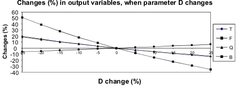
asDchanges are shown inFig. 5.

4.2.3. Implications

Our analysis of the effects of changes in the six unknown parameters values on ATP and the four decision variables –

T;F;Q, andB– leads to two basic conclusions:

1. As is shown for the basic EOQ model in many introductory texts on inventory control model, even relatively large changes in or mis-estimation of the value of a model parameter have rela-tively small effects on the value of the model’s performance measure. Our conclusion here is basically the same. The only model parameter that generated changes in ATP of more than approximately one percent for a parameter change of ±25%

wasb. Thus, if the user’s interest is primarily finding a solution

that will give a value of ATP close to the optimal without wor-rying about whether the values of the decision variables are approximately correct, keeping the parameter estimates within about 25% of the true values should be sufficient.

0

Percent Reduction in ATP When Parameters Are Changed One at a Time

A

Fig. 3.Percent reduction in ATP when parameters are changed one at a time.

0 Reduction in ATP when (1-β) changes

Fig. 4.Change in ATP based on the change in 1b.

Table 5

Direction of changes in decision variable values as a parameter increases. Increase in

parameter

Change in

T F Q B

A Increase Decrease Increase Increase

D Decrease Increase Decrease Decrease

i Decrease Decrease Decrease Increase

g Decrease Increase Decrease Decrease

p Decrease Increase Decrease Decrease

b Nonmonotone Decrease Nonmonotone Increase

Table 4

Sensitivity analysis when parameterbchanges its value (through changes in 1bwith 10% increments).

Change (%) Value Values of variables Changes in variables

1b b T F Q B ATP T(%) F(%) Q(%) B(%) ATP (%)

50 0.90 1.85457 0.684458 347.507 93.6315 623.469 +6.35 14.99 +3.68 +72.19 1.0676

40 0.88 1.84420 0.705254 347.098 86.9714 625.654 +5.76 12.40 +3.56 +59.94 0.7208

30 0.86 1.82852 0.727318 345.759 79.7765 627.482 +4.86 9.66 +3.16 +46.71 0.4307

20 0.84 1.80699 0.750996 343.400 71.9916 628.906 +3.63 6.72 +2.46 +32.39 0.2049

10 0.82 1.77900 0.776732 339.912 63.5511 629.848 +2.02 3.52 +1.42 +16.87 0.0553

+10 0.78 1.70036 0.836901 328.978 44.3722 629.779 2.49 +3.95 1.84 18.40 0.0663

+20 0.76 1.64754 0.873217 321.152 33.4208 628.332 5.52 +8.46 4.18 38.54 0.2960

+30 0.74 1.58376 0.915651 311.408 21.3741 625.446 9.18 +13.73 7.09 60.69 0.7539

+40 0.72 1.50695 0.96665 299.381 8.0411 620.456 13.58 +20.07 10.68 85.21 1.5456

(11)

2. If, on the other hand, the user is equally as interested in having

the values ofT;F;Q, andBbe approximately correct, then less

attention can be paid to estimating the values ofA;g, and

p

and more attention needs to be paid to estimating the values

ofi;D, andb.

One final comment on sensitivity analysis is relevant. Due to the

relative complexity of the equations forTandFand, as a result, for

the ATP, we used, as is most frequently done in assessing the sen-sitivity of a model to changes in its inputs, a numerical approach in

this study. As was pointed out byChu and Chung (2004)in their

discussion of sensitivity analysis of a basic EOQ with partial back-ordering, ‘‘the conclusions made by the analyses of sensitivities based on the computational results of a set of numerical examples are questionable since different conclusions may be made if differ-ent sets of numerical examples are analyzed.’’ While we are confi-dent that our conclusions above are fairly general, any user of this or a similarly complex model needs to conduct his or her own study.

5. Conclusion

We extended the basic EOQ model with incremental discounts by combining the basic solution procedure for that problem with

repeated use ofPentico and Drake’s (2009) models for the EOQ

with full or partial backordering at a constant ratebto determine

the best order quantity for each possible cost. Minimum cost (or maximum profit) was then used to choose among the best full (or partial) backordering solution, meeting all demand and losing all sales. We developed a condition under which partial backorder-ing is optimal and guarantees global optimal values of period length, fraction of demand that will be filled from stock, and order quantity. We illustrated the developed models and proposed solu-tion procedures with examples. A numerical study based on one of the partial backordering example problems was used to evaluate the sensitivity of the model’s results to the changes or mis-estima-tion of the various parameters. Extending the proposed model to include different fixed ordering costs for different price intervals and also considering the pricing issue to determine the optimal selling price of the ordered quantity are some directions for future research.

Funding

The research for the first author was supported by the Iran National Science Foundation (INSF), Fund No. [INSF-93027686].

Appendix A–F. Supplementary material

Supplementary data associated with this article can be found, in

the online version, athttp://dx.doi.org/10.1016/j.cie.2015.01.005.

References

Abad, P. L. (2000). Optimal lot size for a perishable good under conditions of finite production and partial backordering and lost sale. Computers & Industrial Engineering, 38, 457–465.

Archetti, C., Bertazzi, L., & Speranza, M. G. (2014). Polynomial cases of the economic lot sizing problem with cost discounts.European Journal of Operational Research, 237, 519–527.

Bai, Q. G., & Xu, J. T. (2011). Optimal solutions for the economic lot-sizing problem with multiple suppliers and cost structures.Journal of Applied Mathematics and Computing, 37, 331–345.

Benton, W. C., & Park, S. (1996). A classification of literature on determining the lot size under quantity discount.European Journal of Operational Research, 92, 219–238. Bera, U. K., Bhunia, A. K., & Maiti, M. (2013). Optimal partial backordering

two-storage inventory model for deteriorating items with variable demand. International Journal of Operational Research, 16, 96–112.

Chen, S. P., & Ho, Y. H. (2011). Analysis of the newsboy problem with fuzzy demands and incremental discounts.International Journal of Production Economics, 129, 169–177.

Chu, P., & Chung, K.-J. (2004). The sensitivity of the inventory model with partial backorders.European Journal of Operational Research, 152, 289–295.

Chung, C. S., Hum, S. H., & Kirca, O. (1996). The coordinated replenishment dynamic

lot-sizing problem with quantity discounts.European Journal of Operational

Research, 94, 122–133.

Ebrahim, R. M., Razm, J., & Haleh, H. (2009). Scatter search algorithm for supplier selection and order lot sizing under multiple price discount environment. Advances in Engineering Software, 40, 766–776.

Güder, F., Zydiak, J., & Chaudhry, S. (1994). Capacitated multiple item ordering with incremental quantity discounts.Journal of the Operational Research Society, 45,

1197–1205.

Hadley, G., & Whitin, T. M. (1963).Analysis of inventory systems. Englewood Cliffs, NJ, USA: Prentice-Hall International, Inc., USA.

Haksever, C., & Moussourakis, J. (2008). Determining order quantities in multi-product inventory systems subject to multiple constraints and incremental discounts.European Journal of Operational Research, 184, 930–945.

Harris, F. W. (1913). How many parts to make at once.Factory, The Magazine of

Management, 10, 135–136. Reprinted in (1990),Operations Research, 38, 947–950. Hu, J., & Munson, C. L. (2002). Dynamic demand lot-sizing rules for incremental

quantity discounts.Journal of the Operational Research Society, 53, 855–863. Hu, J., Munson, C. L., & Silver, E. A. (2004). A modified silver-meal heuristic for

dynamic lot sizing under incremental quantity discounts. Journal of the

Operational Research Society, 55, 671–673.

Lee, A. H. I., Kang, H. Y., Lai, C. M., & Hong, W. Y. (2013). An integrated model for lot

sizing with supplier selection and quantity discounts. Applied Mathematical

Modelling, 37, 4733–4746.

Lin, C. S., & Kroll, D. E. (1997). The single-item newsboy problem with dual performance measures and quantity discounts.European Journal of Operational Research, 100, 562–565.

Mendoza, A., & Ventura, J. A. (2008). Incorporating quantity discounts to the EOQ model with transportation costs.International Journal of Production Economics, 113, 754–765.

Montgomery, D. C., Bazaraa, M. S., & Keswani, A. K. (1973). Inventory models with a mixture of backorders and lost sales.Naval Research Logistics Quarterly, 20, 255–263. Munson, C. L., & Hu, J. (2010). Incorporating quantity discounts and their inventory

impacts into the centralized purchasing decision. European Journal of

Operational Research, 201, 581–592.

Pentico, D. W., & Drake, M. J. (2009). The deterministic EOQ with partial backordering: A new approach.European Journal of Operational Research, 194, 102–113. Pentico, D. W., & Drake, M. J. (2011). A survey of deterministic models for the EOQ

and EPQ with partial backordering.European Journal of Operational Research, 214, 179–198.

Rieksts, B. Q., Ventura, J. A., Herer, Y. T., & Sun, D. (2007). Technical note: Worst case performance of power of two policies for serial inventory systems with incremental quantity discounts.Naval Research Logistics, 54, 583–587. Rubin, P. A., & Benton, W. C. (2003). Evaluating jointly constrained order quantity

complexities for incremental discounts.European Journal of Operational Research, 149, 557–570.

San José, L. A., Sicilia, J., & García-Laguna, J. (2005). The lot size-reorder level inventory system with customers impatience functions.Computers & Industrial Engineering, 49, 349–362.

Sharma, S., & Sadiwala, C. M. (1997). Effects of lost sales on composite lot sizing. Computers & Industrial Engineering, 32, 671–677.

Stojkovska, I. (2013). Mathematical programming approach to the optimality of the solution for deterministic inventory models with partial backordering.Advances in Operations Research, 2013, 7pages. Article ID 272648.

Taleizadeh, A. A., Barzinpour, F., & Wee, H. M. (2011). Meta-heuristic algorithms for

solving a fuzzy single-period problem.Mathematical and Computer Modelling,

54, 1273–1285.

Taleizadeh, A. A., Niaki, S. T. A., Aryanezhad, M. B., & Fallah-Tafti, A. (2010). A genetic algorithm to optimize multi-product multi-constraint inventory control

systems with stochastic replenishment intervals and discount.International

Journal of Advanced Manufacturing Technology, 51, 311–323.

Taleizadeh, A. A., Niaki, S. T. A., & Hosseini, V. (leizadeh et al., 2009). Optimizing multi product multi constraints bi-objective newsboy problem with discount

by hybrid method of goal programming and genetic algorithm.Engineering

Optimization, 41, 437–457.

-40

Changes (%) in output variables, when parameter D changes

T

F

Q

B

Fig. 5.Percent changes inT;F;Q, andBwhenDchanges by a given percent.

(12)

Taleizadeh, A. A., Niaki, S. T. A., & Nikousokhan, R. (2011). Constraint multiproduct joint-replenishment inventory control problem using uncertain programming. Applied Soft Computing, 11, 5134–5154.

Taleizadeh, A. A., & Pentico, D. W. (2014). An economic order quantity model with partial backordering and all-units discount.International Journal of Production Economics, 155, 172–184.

Taleizadeh, A. A., Wee, H. M., & Sadjadi, S. J. (2010). Multi-product production quantity model with repair failure and partial backordering. Computers & Industrial Engineering, 50, 45–54.

Tersine, R. J. (1994).Principles of inventory and materials management(4th ed.). Englewood Cliffs, NJ, USA: Prentice-Hall International, Inc., USA.

Tersine, R. J., & Toelle, R. A. (1985). Lot size determinations with quantity discounts. Production and Inventory Management, 26(3), 1–23.

Wee, H.-M. (1993). Economic production lot size model for deteriorating items with partial back-ordering.Computers & Industrial Engineering, 24, 449–458. Weng, Z. K. (1995). Modeling quantity discounts under general price-sensitive

demand functions: Optimal policies and relationships. European Journal of