COMPARISON OF 3D POINT CLOUDS FROM AERIAL STEREO IMAGES AND LIDAR
FOR FOREST CHANGE DETECTION
D. Ali-Sisto1, *, P. Packalen1
1 School of Forest Sciences, Faculty of Science and Forestry, University of Eastern Finland, P.O. Box 111, 80101 Joensuu, Finland –(daniela.ali-sisto, petteri.packalen)@uef.fi
Commission III, WG III/1
KEY WORDS: Change detection, forestry, image matching, image point cloud, LiDAR, Semi-Global Matching (SGM)
ABSTRACT:
This study compares performance of aerial image based point clouds (IPCs) and light detection and ranging (LiDAR) based point clouds in detection of thinnings and clear cuts in forests. IPCs are an appealing method to update forest resource data, beca use of their accuracy in forest height estimation and cost-efficiency of aerial image acquisition. We predicted forest changes over a period of three years by creating difference layers that displayed the difference in height or volume between the initial and subsequent time points. Both IPCs and LiDAR data were used in this process. The IPCs were constructed with the Semi-Global Matching (SGM) algorithm. Difference layers were constructed by calculating differences in fitted height or volume models or in canopy height models (CHMs) from both time points. The LiDAR-derived digital terrain model (DTM) was used to scale heights to above ground level. The study area was classified in logistic regression into the categories ClearCut, Thinning or NoChange with the values from the difference layers. We compared the predicted changes with the true changes verified in the field, and obtained at best a classification accuracy for clear cuts 93.1% with IPCs and 91.7% with LiDAR data. However, a classification accuracy for thinnings was only 8.0% with IPCs. With LiDAR data 41.4% of thinnings were detected. In conclusion, the LiDAR data proved to be more accurate method to predict the minor changes in forests than IPCs, but both methods are useful in detection of major changes.
* Corresponding author
1. INTRODUCTION
Airborne light detection and ranging (LiDAR) and aerial images are widely used data sources in forest inventories. With LiDAR data it is possible to obtain very accurate estimates for height-dependent stand variables (Hyyppä et al., 2008; Lim et al., 2003; Wulder et al., 2012). In Finland, LiDAR data is acquired by Finnish Forest Centre and National Land Survey of Finland (NLS) at intervals of ten years (Maltamo et al., 2011). However, collecting point clouds with LiDAR technology is somewhat expensive whereupon more cost-effective alternatives to generate 3D point clouds are appealing. There can also be need to update forest data in more often than every tenth year when new LiDAR data is collected. Aerial imaging is one way to gather aerial remote sensing data with lower costs than with LiDAR.
Recent years methods to generate 3D image point clouds (IPCs) from aerial stereo images have been under intensive development. Because of better image matching algorithms, increasing computing capacity and improving quality of aerial images, usability of IPCs in forest inventory has been realized. Remote sensing data can be acquired for forestry purposes with the fraction of costs if only aerial images are needed instead of both airborne LiDAR data and aerial images. IPC data is more or less comparable to airborne LiDAR data since both characterize forest dimensions in 3D (Leberl et al., 2010). The major difference is that LiDAR provides more accurate terrain
model (DTM)(Ackermann, 1999; Lee and Younan, 2003; Su and Bork, 2006). Because IPC is a very appealing data source, its use in forestry has recently been increasingly examined (Gobakken et al., 2015; Järnstedt et al., 2012; Nurminen et al., 2013; Rahlf et al., 2014; Stepper et al., 2015).
Forest change detection yields information of changes in forest structure. Changes can result from natural or human induced disturbances such as storms, clear cuts or thinnings. Most changes cause canopy gaps. Change detection is therefore an appealing application for IPCs, because IPCs represent canopy structure in a very detailed way, which enables detection of small gaps in the canopy. Change detection in forests has traditionally based on the visual interpretation of aerial images, but because of the laboriousness and subjectivity of this method, the use of aerial imagery in automatic forest change detection has been widely investigated (Coppin et al., 2004; Hussain et al., 2013). However, the use of aerial imagery in the detection of thinnings is somewhat problematic, because they mainly yield information on changes at the top of the canopy.
reliability of forest resource data, even if the accuracy is not as good as with LiDAR data. In this study, we evaluate the accuracy of IPC-based forest change detection in comparison with LiDAR based change detection.
2. MATERIAL
The study area of 36 km2 was located in Juuka, Eastern Finland. We used two sets of aerial stereo images, LiDAR data and field data in this study. Twenty overlapping aerial images were obtained on 1 May 2009 at the height of 5100 m with the Z/I DMC camera. Ground sampling distance was 50 cm, sidelap 30% and endlap 60%. 36 overlapping aerial images were obtained on 12 June 2013 at the height of 5900 m with the Microsoft Ultracam Xp camera. Ground sampling distance was 35 cm, sidelap 45% and endlap 80%.
LiDAR data for generation of DTM were obtained on 14 May 2010 at the height of 2250 m with the Leica ALS60 scanner and pulse density of 0.87 points/m2. Another set of LiDAR data were obtained on 25 July 2013 at the height of 1900 m with the Leica ALS70 scanner and pulse density of 0.75 points/m2 for measurement were predicted with the H-D curve of Eerikäinen (Eerikäinen, 2009). For validation of the used method, another set of field data was collected between 29 September and 17 October 2014 by recording whether thinnings or clear cuts had been performed. Only those stands in which clear cuts and thinnings were possibly taken place were checked, because we had as many as 2558 forest stands. Selection of stands to be
The detection of thinned and clear-cut areas was performed by examining the relative change in stand height and volume between the years 2009/2010 and 2013 by using IPC and LiDAR data and a LiDAR-derived DTM. We created IPCs from overlapping aerial stereo images with the Semi-Global Matching (SGM) (Hirschmüller, 2005) algorithm.
Image matching algorithms require that there are two or more overlapping images under the area of interest. If the same object can be observed at least in two overlapping images on the basis of cross-correlation between images and the interior and exterior orientation of the images are known, height of the
object can be determined. 3D point clouds are created by repeating this in every pixel or pixel groups in the images. SGM combines global and local stereo methods in pixel-wise matching. Corresponding points are found by minimizing the Mutual Information based matching cost in pixels and aggregating it with several 1D path directions on the image. In this study, we used ERDAS IMAGINE’s SGM implementation, which is available in the AutoDTM module. SGM was executed with three spectral bands, red, green, and created difference layers that displayed the relative difference in height or volume between the years 2009/2010 and 2013. These difference layers were constructed using two different approaches. The first one was based on the use of canopy height models (CHM) and the second one on the use of local IPC-based Lorey’s height and volume models.
CHMs were created by using the CanopyModel program in the FUSION toolset (McGaughey, 2014). The function set the pixel values in CHMs to depict the height of the highest point within the 17 m 17 m pixel area. The DTMs were used to scale pointwise elevations to heights above ground level prior to determination of the highest point. If there were no points for a pixel, the height value was set to NoData. As the final step, a median filter was applied with a 3 3 neighbourhood in order to remove NoData pixels from CHMs and to produce a slightly smoothed surface.
Lorey’s height and volume models were fitted with a linear regression model in the R platform (R Core Team, 2012). The field measured plotwise volumes or heights from the year 2013 were used as dependent variables, and height metrics calculated from IPCs and LiDAR data with FUSION’s CloudMetrics program were used as predictor variables. Stepwise variable selection, which is based on the use of Akaike’s information criterion (Akaike, 1973; Burnham and Anderson, 2002), was used in the selection of the best predictors from the 99 possible IPC variables with the step function in R. The best model forms were selected based on the root mean square error (RMSE). Lorey’s height and volume models were then used to predict heights and volumes for the raster of 17 m 17 m that covered the whole study area. = height or volume estimated from the IPCs n = number of sample plots
This was done by dividing the values in 2013 rasters by the corresponding values in 2009/2010 rasters. The values from the difference layers were then used in multinomial logistic regression models with the multinom function from the nnet
package (Ripley, 2016) in R in order to classify the pixels in study area into the categories ClearCut, Thinning or NoChange.
Predictor variable Abbreviation
Difference in volumes predicted with 2009 and 2013 SGM (blue band) ve_sgm1
Difference in volumes predicted with 2009 and 2013 SGM (green band) ve_sgm2
Difference in volumes predicted with 2009 and 2013 SGM (red band) ve_sgm3
Difference in CHMs created with 2009 and 2013 SGM1 sgm1
Difference in CHMs created with 2009 and 2013 SGM2 sgm2
Difference in CHMs created with 2009 and 2013 SGM1 sgm3
Difference in CHMs created with 2010 and 2013 LiDAR las
Difference in volumes predicted with 2009 and 2013 LiDAR ve_las
Difference in heights predicted with 2009 and 2013 LiDAR he_las
Table 2. The most important predictor variables and their abbreviations.
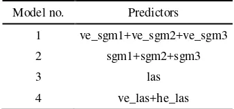
Model no. Predictors
1 ve_sgm1+ve_sgm2+ve_sgm3
2 sgm1+sgm2+sgm3
3 las
4 ve_las+he_las
Table 3. The model numbers and predictor variables (explained in Table 2) in the selected models.
Field-measured change information was utilized as dependent variable in these models. The best predictors (Table 2, 3) were selected with stepwise variable selection.
The pixelwise results were aggregated to the stand level by selecting the most suitable category utilizing proportions of different categories in the stand area. First we specified threshold values to the categories ClearCut and Thinning that maximized classification accuracy. If the category ClearCut covered higher proportion of the stand area than the threshold value, it was chosen. If not, we chose the category Thinning, if its coverage exceeded the threshold. Otherwise, we chose the category NoChange. Accuracy assessment was performed with the confusion matrix, overall accuracy and Cohen’s kappa (Cohen, 1960).
4. RESULTS
Change detection was performed with CHM-based method or height and volume model based method. The results were better with the latter. When thinnings and clear cuts were compared with the true changes verified in the field (Table 4) by using height and volume model based method, we obtained
a stand level classification accuracy for clear cuts being 79.2% with IPCs, but only 8.0% for thinnings. At pixel level results were worse. Only 58.1% of clear cuts and 0.9% of thinnings were detected. With LiDAR data classification accuracies were higher; as much as 91.7% of clear cuts and 41.4% of thinnings were detected at stand level and 77.0% of clear cuts and 6.8% of thinnings were detected at pixel level.
With CHM-based method thinnings were not detectable at all regardless of the data source. With IPCs, 93.1% of clear cuts were detected at stand level and 65.2% at pixel level. With LiDAR data, 88.9% of clear cuts were detected at stand level and 62.5% at pixel level. Kappa coefficients were rather low in every case (Table 5), indicating high influence of random chance on the results.
5. DISCUSSION
Our method proved to be reliable in detection of clear cuts. With IPCs, we could detect nearly all clear cuts from aerial images, and with LiDAR data detection accuracy was equally good. These results were expected, because clear cuts were also visually observable in aerial images. However, detection accuracy of thinnings was much lower. With IPCs we could locate at best 8.0% of stands, in which thinnings were performed. With LiDAR data results were better and 41.4% of thinnings were detected at best.
thinnings succeeded rather well, possibly because with LiDAR it is possible to obtain more reliable information of lower parts of the canopy.
Volume models seemed to be the best way to detect thinnings, possibly because low thinnings influence more to the volume of
growing stock than to forest height. With CHM-based difference layers we were not able to detect any of the thinnings regardless of the data source.
A True B True
NoChange Thinning ClearCut NoChange Thinning ClearCut
NoChange 99.5 98.4 41.7 99.3 92.0 20.8
Thinning 0.0 0.9 0.1 0.2 8.0 0.0
ClearCut 0.5 0.7 58.1 0.5 0.0 79.2
C True D True
NoChange Thinning ClearCut NoChange Thinning ClearCut
NoChange 99.4 99.3 34.8 98.9 100.0 6.9
Thinning 0.0 0.0 0.0 0.0 0.0 0.0
ClearCut 0.6 0.7 65.2 1.1 0.0 93.1
E True F True
NoChange Thinning ClearCut NoChange Thinning ClearCut
NoChange 99.1 92.8 13.5 97.0 58.6 5.6
Thinning 0.5 6.8 9.5 2.4 41.4 2.8
ClearCut 0.4 0.3 77.0 0.7 0.0 91.7
G True H True
NoChange Thinning ClearCut NoChange Thinning ClearCut
NoChange 98.8 96.0 37.5 99.0 100.0 11.1
Thinning 0.0 0.0 0.0 0.0 0.0 0.0
ClearCut 1.2 4.0 62.5 1.0 0.0 88.9
Table 4. Confusion matrix for predictions for the categories ClearCut, thinning, and NoChange. Values are percentages. (A) Pixel -level predictions made with model 1. (B) Stand--level predictions made with model 1. (C) Pixel--level predictions made with model 2. (D) Stand-level predictions made with model 2. (E) Pixel-level predictions made with model 3. (F) Stand-level predictions made
with model 3. (G) Pixel-level predictions made with model 4. (H) Stand-level predictions made with model 4.
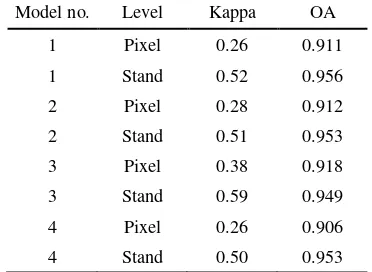
Model no. Level Kappa OA
1 Pixel 0.26 0.911
1 Stand 0.52 0.956
2 Pixel 0.28 0.912
2 Stand 0.51 0.953
3 Pixel 0.38 0.918
3 Stand 0.59 0.949
4 Pixel 0.26 0.906
4 Stand 0.50 0.953
Table 5. The kappa coefficients and overall accuracies (OA) of the best models at the pixel and stand level.
6. CONCLUSIONS
Altogether, we could predict minor changes in forest more reliably with LiDAR data than with IPCs, but major changes were predicted almost equally reliably. The most of the clear
cuts were detected both with IPCs and LiDAR data, but thinnings were more difficult to locate. With LiDAR data we could detect almost half of the thinnings, but with IPCs only small part of the thinnings were detected.
Estimation of growing stock volume proved to be the best method to detect occurred changes in forests regardless of the data source. Although IPCs were not very effective in detection of thinnings, we can assume that IPCs are useful in other height-related forestry applications in which LiDAR data is traditionally used.
REFERENCES
Ackermann, F., 1999. Airborne laser scanning-present status and future expectations. ISPRS J. Photogramm. Remote Sens. 54, 64–67.
Burnham, K., Anderson, D., 2002. Model Selection and Multimodel Inference: A Practical Information-Theoretic Approach, 2nd ed. Springer-Verlag, New York, NY, USA.
Cohen, J., 1960. A Coefficient of Agreement for Nominal Scales. Educ. Psychol. Meas. 20, 37–46.
Coppin, P., Jonckheere, I., Nackaerts, K., Muys, B., Lambin, E., 2004. Digital change detection methods in ecosystem monitoring: a review. Int. J. Remote Sens. 25, 1565–1596.
Eerikäinen, K., 2009. A multivariate linear mixed-effects model for the generalization of sample tree heights and crown ratios in the Finnish National Forest Inventory. For. Sci. 55, 480–493.
Gobakken, T., Bollandsås, O.M., Næsset, E., 2015. Comparing biophysical forest characteristics estimated from photogrammetric matching of aerial images and airborne laser scanning data. Scand. J. For. Res. 30, 73–86.
Hirschmüller, H., 2005. Accurate and efficient stereo processing by semi-global matching and mutual information. IEEE Int. Conf. Comput. Vis. Pattern Recognit. 2, 807–814.
Hussain, M., Chen, D., Cheng, A., Wei, H., Stanley, D., 2013. Change detection from remotely sensed images: From pixel-based to object-pixel-based approaches. ISPRS J. Photogramm. Remote Sens. 80, 91–106.
Hyyppä, J., Hyyppä, H., Leckie, D., Gougeon, F., Yu, X., Maltamo, M., 2008. Review of methods of small-footprint airborne laser scanning for extracting forest inventory data in boreal forests. Int. J. Remote Sens. 29, 1339–1366.
Isenburg, M., 2015. LAStools - efficient tools for LiDAR
processing [WWW Document]. URL
http://rapidlasso.com/lastools/ (accessed 9.28.16).
Järnstedt, J., Pekkarinen, A., Tuominen, S., Ginzler, C., Holopainen, M., Viitala, R., 2012. Forest variable estimation using a high-resolution digital surface model. ISPRS J. Photogramm. Remote Sens. 74, 78–84.
Leberl, F., Irschara, A., Pock, T., Meixner, P., Gruber, M., Scholz, S., Wiechert, A., 2010. Point Clouds: Lidar versus 3D Vision. Photogramm. Eng. Remote Sens. 76, 1123–1134.
Lee, H.S., Younan, N.H., 2003. DTM extraction of Lidar returns via adaptive processing. IEEE Trans. Geosci. Remote Sens. 41, 2063–2069.
Lim, K., Treitz, P., Wulder, M., St-Onge, B., Flood, M., 2003. LiDAR remote sensing of forest structure. Prog. Phys. Geogr. 27, 88–106.
Maltamo, M., Packalén, P., Kallio, E., Kangas, J., Uuttera, J., Heikkilä, J., 2011. Airborne laser scanning based stand level management inventory in Finland, in: Proc. SilviLaser 2011, 11th Int.Conf. LiDAR Applications for Assessing Forest Ecosystems. Hobart, Australia, pp. 1–10.
McGaughey, R.J., 2014. FUSION/LDV: Software for LIDAR data analysis and visualization. USDA.
Nurminen, K., Karjalainen, M., Yu, X., Hyyppä, J., Honkavaara, E., 2013. Performance of dense digital surface models based on image matching in the estimation of plot-level forest variables. ISPRS J. Photogramm. Remote Sens. 83, 104– 115.
R Core Team, 2012. A Language and Environment for Statistical Computing [WWW Document]. URL https://cran.r-project.org/doc/manuals/r-release/fullrefman.pdf (accessed 9.28.16).
Rahlf, J., Breidenbach, J., Solberg, S., Næsset, E., Astrup, R., 2014. Comparison of four types of 3D data for timber volume estimation. Remote Sens. Environ. 155, 325–333.
Ripley, E., 2016. Package “nnet” [WWW Document]. URL https://cran.r-project.org/web/packages/nnet/nnet.pdf (accessed 9.28.16).
Stepper, C., Straub, C., Pretzsch, H., 2015. Using semi-global matching point clouds to estimate growing stock at the plot and stand levels: application for a broadleaf-dominated forest in central Europe. Can. J. For. Res. 123, 111–123.
Su, J., Bork, E., 2006. Influence of vegetation, slope, and lidar sampling angle on DEM accuracy. Photogramm. Eng. Remote Sensing 72, 1265–1274.
Wulder, M.A., White, J.C., Nelson, R.F., Næsset, E., Ørka, H.O., Coops, N.C., Hilker, T., Bater, C.W., Gobakken, T., 2012. Lidar sampling for large-area forest characterization: A review. Remote Sens. Environ. 121, 196–209.
This paper is based on the following paper: