EFFECTS OF TILT AND AZIMUTH ON ANNUAL INCIDENT SOLAR RADIATION

Proceedings of Solar Forum 2001: Solar Energy: The Power to Choose April 21-25, 2001, Washington, DC

EFFECTS OF TILT AND AZIMUTH ON ANNUAL INCIDENT SOLAR RADIATION

FOR UNITED STATES LOCATIONS

Craig B. Christensen

National Renewable Energy Laboratory 1617 Cole Blvd.

Golden, CO 80401 e-mail: craig_christensen@nrel.gov

Greg M. Barker Mountain Energy Partnership

3227 Ridge Road Nederland, CO 80466 e-mail: GBarker123@aol.com

ABSTRACT

This paper presents generalized results regarding the effect of surface orientation on annual incident solar radiation for locations in the United States. A surface-orientation factor (SOF) is defined, equal to Iann/Iann,max, the

ratio of annual incident solar radiation for a particular orientation to annual incident solar radiation for an optimally oriented surface.

SOF contour plots can be used to conveniently indicate the effects of surface orientation over a range of tilt and azimuth angles (from horizontal to vertical and from south to east/west). Correlations, presented in this paper, can be used to calculate SOF’s based on latitude and a climate factor, w. Regional SOF contour plots indicate surface orientation effects by geographic region with boundaries determined according to latitude-w values. Effects of morning/afternoon cloudiness and snow cover are also addressed.

NOMENCLATURE

Az surface azimuth angle: the angle between true south and the projection on a horizontal plane of the normal to the surface (degrees), -90o = east , +90o = west

Azopt optimal surface azimuth angle: the azimuth

angle at which the annual incident solar radiation on an optimally tilted surface is maximized (degrees)

SOF surface orientation factor: Iann/Iann,max

SOFhor SOF for a horizontal surface

SOFs SOF for a south-facing surface

SOFs,lat SOFs for a surface with tilt=latitude

Iann annual incident solar radiation on a surface with

any orientation (MJ/m2 year)

Iann,lat Iann for a south-facing surface with tilt=latitude

(MJ/m2 year)

Iann,hor Iann for a horizontal surface (MJ/m 2

year)

Iann,max Iann for a south-facing surface with optimal tilt

(MJ/m2 year)

Kt,ann annual average clearness index; the ratio of

terrestrial radiation to extraterrestrial radiation, on a horizontal surface

Kt,sum summer (May, June, and July) average

clearness index

Kt,win winter (November, December, and January)

average clearness index

L north latitude (degrees)

T surface tilt angle from horizontal (degrees)

Topt optimal surface tilt angle : the angle at which

the annual incident solar radiation on a south-facing surface is maximized (degrees)

w a climate-dependent factor to adjust for the difference between tilt=latitude and optimal tilt for a south-facing surface (degrees)

INTRODUCTION

annual incident solar radiation is reduced for non-optimal surface orientations.

Computer-based solar design tools can be used to quickly evaluate the effect of a specific surface orientation (tilt/azimuth) in a particular geographic location. However, it is sometimes useful to have more general information (e.g., for a wide range of collector orientations and/or geographic locations) available without needing to perform specific computer runs.

BACKGROUND

Previous studies (Morse and Czarnecki, 1958; Duffie and Beckman, 1991; Willmott, 1982) indicate the sensitivity to surface orientation, giving total annual incident solar radiation as a function of tilt and azimuth angle for selected locations. ASHRAE (1997) gives tabular data for clear-day solar irradiance by month for vertical surfaces for 16 azimuth angles as a function of latitude.

General “rules of thumb” exist. For maximum annual incident solar radiation, for example, conventional wisdom says that: 1) a south-facing (in the northern hemisphere) surface with tilt equal to latitude is best, and 2) deviations in azimuth angles of 10o or 20o from south have small effect.

In the 1970’s and 1980’s, in an attempt to adhere to the rules of thumb and achieve near-optimal collector orientation, many solar energy system installations involved rack-mounted collectors at complicated angles to the roof. Early interest in active solar space heating focussed attention on steep collector tilts (due to seasonal operation and northern latitudes) and relatively low tolerance for off-south azimuth angles.

Today, more flexibility and simpler installations are desired. The information presented in this paper indicates that surface tilt angles and azimuth angles can be varied over a considerable range without significantly reducing the amount of annual incident solar radiation. This is especially true for locations with low latitudes and typical low-angle roof tilts (i.e., 20o to 30o).

METHODOLOGY

A database was developed of annual incident solar radiation values for surfaces at various tilt and azimuth angles for 239 TMY2 locations in the United States. The values in the database were calculated by processing TMY2 data (Marrion, 1995) using the Type 16 solar radiation processor in the TRNSYS simulation program (Klein, et al, 1996) with the Perez anisotropic diffuse radiation model (Perez, et al, 1988). The horizon was assumed to be unobstructed by buildings, trees or other objects. In general, ground reflectance was fixed at 0.2 for

all locations at all times of the year. See discussion on the effect of snow cover in the Results section.

Annual incident solar radiation values were calculated for azimuths ranging from east to west in 15 degree increments, and for tilts from horizontal to vertical in 15 degree increments. For developing SOF correlations, values for non-south orientations are the average of values for orientations on either side of south (e.g., values for 30o east and 30o west, averaged). See discussion on the effect of morning/afternoon cloudiness in the Results section.

To find optimal tilts (at which the annual incident solar radiation is maximized) for surfaces facing due south, a second-order equation of the form:

Iann = a0 + a1 T + a2 T2 (1)

was fit for each location using a least-squares regression, with tilts ranging from 0 to 75 degrees at 7.5-degree increments. The optimal tilt was then calculated as the tilt at which the first derivative of Eq. 1 is equal to zero:

Topt = - a1/(2 a2) (2)

This method was checked for all TMY2 locations by running TRNSYS simulations at one-degree increments of tilt in the vicinity of the Topt values from Eq. (2). The Topt

values from Eq. (2) were within less than 1 degree of the values from TRNSYS for all locations. Optimal azimuth was calculated using a similar method, this time fitting an equation for Iann as a function of azimuth for a surface tilted

at Topt and finding the azimuth at which the derivative is

equal to zero.

APPROACH

1. Surface Orientation Factors

For a given geographic location, it is useful to see how incident solar radiation is reduced if a surface is not at the optimal orientation. For this purpose, we define a surface orientation factor (SOF) as:

SOF = Iann/Iann,max (3)

where Iann is the annual incident solar radiation on a surface

with a particular orientation and Iann,max is the annual

-90 -60 -30 0 30 60 90

Fig. 1: Correlation-based SOF contour plot

[ = optimal orientation, ___ = 0.95 SOF]

There are several ways to obtain a SOF contour plot for a particular location. First, annual incident solar radiation values can be calculated directly from hourly data for the full range of tilt and azimuth angles and used to calculate SOF values for generating a contour plot. Second, correlations developed in this paper can be used to calculate SOF values for a contour plot. Third, one of several regional SOF contour plots given in this paper can be selected as reasonably representative for the particular location.

2. South-Facing Surfaces

To develop SOF correlations, we begin by examining annual incident solar radiation as a function of surface tilt for surfaces facing due south. Figure 2 shows values for selected geographic locations. As expected, the results vary in both magnitude and sensitivity to tilt.

0.0

Fig. 2: Annual incident solar radiation versus tilt

To create surface orientation factors for south-facing surfaces (SOFs), the values in Fig. 2 were normalized by

dividing by Iann,max

,

the maximum annual incident solar

radiation value, for each location, and results are shown in

Fig. 3. The results are plotted versus (tilt – latitude) in an attempt to align the curves left-to-right. If the usual assumption of optimal tilt equal to latitude were correct, the maximums in Fig. 3 would occur at (tilt – latitude) equals zero. However, the maximums (and the curves) are not well-aligned, indicating that the typical assumption of optimal tilt equals latitude is imperfect.

0.0

Tilt - Latitude (degrees)

SOF

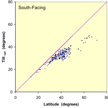
Optimal surface tilt angles (for maximum annual incident solar radiation) versus latitude are shown in Fig. 4 for the 239 TMY2 locations geographic locations in the database. Optimal tilts are less than latitude and do not correlate linearly with latitude.

0

Fig. 4: Optimal tilt versus latitude

In order to develop a better correlation, it is useful to understand the reasons that optimal tilts are less than latitude. The basic logic for Topt = L stems from: 1) a

2) a horizontal surface at the equator will have maximum annual incident solar radiation (if there is no seasonal bias in clearness).

Fig. 6: Values of ‘w’ as a function of location 4

8

0

12 12

16

However, for locations away from the equator, there are several possible reasons for lower optimal tilt angles. First, weather is typically clearer during the summer when the sun is higher in the sky. Second, there is more sky diffuse solar radiation incident on surfaces at lower tilt angles. Third, there is less atmospheric attenuation when the sun is higher in the sky. Fourth, lower tilt angles reduce the number of hours when the sun is behind the plane of the surface (at the beginning and end of the day, during the summer).

For south-facing surfaces, the optimal tilt angle (for maximum annual incident solar radiation) may be

estimated as: Figure 7 shows that SOFs values for the 239 TMY2

locations are well correlated with T-(L-w), essentially eliminating the misalignment seen in Fig. 3.

Topt = L-w (4)

The upper out-lying points in Fig. 7 are for a few locations at very high or low latitudes (i.e., in Alaska and Guam). At very low latitudes, vertical south-facing surfaces are an extreme case, receiving little incident solar radiation and leading to discrepancies in SOF values. where the climate-specific factor, w, is given by:

w = 20.6 (1 – Kt,win/Kt,sum) + (0.621 – Kt,ann) L (5)

where Kt,win , Kt,sum and Kt,ann are average clearness indices

for winter (November, December and January), summer (May, June and July) and annually (all 12 months), respectively. The form of Eq. (5) was chosen to reflect the factors described in the previous paragraph while assuring that ‘w’ would equal zero under totally clear conditions at latitude = 0. The coefficients were determined to provide the best fit in Eq. (4) for south-facing surfaces in 239 TMY2 locations as shown in Fig. 5.

0.0 0.2 0.4 0.6 0.8 1.0 1.2

-60 -30 0 30 60 90

Tilt - (Latitude - w) (degrees)

SO

Fs

South-Facing

0 20 40 60

0 20 40 60

Latitude - w (degrees)

T

iltopt

(

d

egrees)

South-Facing

Fig. 7: SOFs versus tilt - (latitude – w)

[RMS error = 0.00874; 3,107 points]

The results in Fig. 7 can be described by:

SOFs = 2.0 – [1.0 + 0.000242 (T-(L-w)) 2

]1/2 (6)

where the form of Eq. 6 was chosen to fit the data with and inverted hyperbola with a maximum value of 1.0.

Fig. 5: Optimal tilt versus (latitude – w)

3. General SOF Correlations [RMS error = 1.21 degrees]

Fitting all the points in the database (the full range of tilt and azimuth angles, for 239 TMY2 locations) using the location-specific correlating variable, L-w, and the definitions in Eq. (5) and (6), gives:

SOF = SOFs

+

{

[b1 + b2 (L-w) + b3 (L-w)2] Az2 + b4 Az3

}

T

+ (b5 Az 2

+ b6 Az 3

) T2 (7)

where

Az = surface azimuth angle (degrees) T = surface tilt angle (degrees)

b1 = -4.97 E-07 b4 = 3.33 E-09

b2 = -3.33 E-08 b5 = 1.30 E-08

b3 = 2.67 E-10 b6 = -4.61 E-11

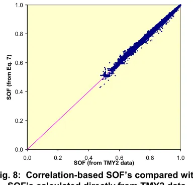
The form of Eq. 7 omits the linear azimuth term to ensure that the slope of SOF contours will be zero where azimuth equals zero (so that there is no inflection point). The goodness-of-fit for this relationship (for the full range of tilt and azimuth angles for 239 TMY2 locations) is indicated by Fig. 8.

0.0 0.2 0.4 0.6 0.8 1.0

0.0 0.2 0.4 0.6 0.8 1.0

SOF (from TMY2 data)

S

O

F (

fr

om

E

q

. 7

)

Fig. 8: Correlation-based SOF’s compared with SOF’s calculated directly from TMY2 data

[RMS error = 0.00886; 11,711 points]

In general, the out-lying points to the right in Fig. 8 correspond with the upper out-lying points in Fig. 7 (where the TMY2 values are higher than the best-fit curve).

RESULTS

1. Regional SOF Contour Plots

Figure 9 shows regional SOF contour plots and geographic regions where they apply based on L–w values. To use the plots in Fig. 9, the user identifies the L-w region in which his location lies by looking at the U.S. map, which is divided into four L-w regions. The corresponding contour plot is then selected, and the SOF vlaue is read at the intersection of the surface tilt and azimuth. If a location is near the contour line between two regions on the U.S. map, then the SOF may be taken as the mean of the SOF’s

from the two corresponding plots. More sophisticated graphical interpolation is probably not warranted. If a more precise measure of SOF is required, then one can use Eqs. 5 and 7 or an hourly simulation tool.

Comparing regional SOF contour plots shows the sensitivity of surface orientation effects as a function of location. For example, for a tilt angle of 26.5 o (a typical 6/12 roof pitch), for a surface to have a SOF greater than 0.9 the surface azimuth may range from 0o to +/-90o for locations with an L-w value of 18, whereas the azimuth must be within 40o of south for a location with an L-w value of 48. For a vertical surface with an azimuth angle 90o from south (i.e., facing east or west), a SOF of approximately 0.55 applies in all locations

2. Optimal Surface Tilt Angles

The U.S. map shown in Fig. 9 is provided to indicate the regions where different SOF plots apply. However, the map also shows optimal tilt angles (Topt = L – w) for

south-facing surfaces.

In many locations, optimal surface tilt angles are significantly lower that the conventional assumption of tilt equal to latitude. This is especially so for locations with cloudy winter weather, while locations in the mountain west, with relatively clear winter weather, show the least difference. For example, note that optimal surface tilt angles are similar for Seattle and Phoenix (approximately 33o).

3. Effect of Morning/Afternoon Cloudiness

For locations where incident solar radiation differs significantly from morning to afternoon, SOF values (if calculated directly from location-specific hourly data) will show differences for east/west surface orientations. For such locations, SOF contour plots based directly on hourly data will show a shift to the east or west. For example, Fig. 10 shows a SOF contour plot based on TMY2 data for Boulder, Colorado where afternoons tend to be cloudy (and there are mountains to the west).

-90 -60 -30 0 30 60 90 0 30 60 90

Azimuth

Tilt Alaska L-w = 48

24 30 36 42

-90 -60 -30 0 30 60 90

0 30 60 90

-90 -60 -30 0 30 60 90

0 30 60 90

-90 -60 -30 0 30 60 90

0 30 60 90

-90 -60 -30 0 30 60 90

0 30 60 90

-90 -60 -30 0 30 60 90

0 30 60 90 Azimuth

Tilt L-w = 42

Azimuth

Tilt Hawaii L-w = 18

Azimuth

Tilt L-w = 36

Azimuth

Tilt L-w = 30

0.5-0.6 0.6-0.7 0.7-0.8 0.8-0.9 0.9-1.0

Azimuth

Tilt L-w = 24

-90 -60 -30 0 30 60 90 0 30 60 90

Azimuth

Tilt Boulder, CO

0.4-0.5 0.5-0.6 0.6-0.7 0.7-0.8 0.8-0.9 0.9-1.0

Fig. 10: TMY2-based SOF contour plot

[ = optimal orientation, ___ = 0.95 SOF]

Figure 11 shows the optimal surface azimuth angle, Azopt, (based on the location-specific hourly data in the

database) for locations where the difference from south is greater than 5o. For annual incident solar radiation, as reported here, there is little difference for most locations. On a seasonal basis, the differences would likely be greater.

-10 -5 0 5 10 15

Fig. 11: Optimal azimuth angle (degrees) [east = - and west = +]

To approximately account for east/west effects, correlation-based SOF contour plots (as in Fig. 9) can be adjusted by shifting the labels on the azimuth axis so that the Azopt value (from Fig. 11) is aligned with the maximum

point on the contour plot.

DISCUSSION

This section discusses interpretation and use of the results presented in the previous section. In general, surface orientation factors are intended for use in preliminary design and/or generalized geographic assessments. A user may use surface orientation factors for preliminary evaluations and then use a design tool with monthly (or hourly) calculations for more detailed analysis.

Any shading effects from objects such as surrounding trees or buildings are not included in the SOF, and would

best be investigated through use of a detailed description of the horizon and an hourly simulation tool.

1. Incident Energy versus Useful Energy

Incident energy is not the same as useful delivered energy, and the surface orientation leading to maximum output of a solar energy system may be quite different from the orientation leading to maximum incident energy. Annual incident solar radiation (and the use of SOF’s) is a useful starting point for estimating energy savings for some, but not all, types of solar energy systems. Strictly speaking, system efficiency needs to be constant throughout the year for the use of annual incident solar radiation and SOF’s to apply.

For solar space heating, for example, the seasonal variation in load is so great (zero during the summer) that annual incident solar radiation is obviously not the appropriate input for available energy. Performance prediction for such systems typically requires at least month-by-month analysis. Therefore, an annual SOF contour plot would not typically be useful for analysis of a solar space heating application.

For solar water heating systems, however, a recent study (Christensen and Barker, 1998) has found that annual efficiencies (calculated as delivered energy over incident energy) are essentially independent of location, so long as the system size is not too large relative to the hot water load (i.e., annual solar fractions less than 0.80). This indicates that, for these types of systems, annual SOF’s may be applicable (seasonal differences in efficiency may be a secondary issue). Many photovoltaic systems also have relatively constant efficiencies throughout the year, so if the per-unit value of the energy savings is also relatively constant, then annual SOF’s may be useful for these types of systems.

2. Solar Radiation Data for Use with SOF’s

SOF’s indicate relative differences in annual incident solar radiation for different surface orientations. However, if the actual value of annual incident solar radiation for a particular surface orientation, Iann, is desired, it can be

obtained form:

Iann = SOF * Iann,max (8)

There are several options for obtaining Iann,max values.

For locations where ‘w’ is not small, Iann can by found

from:

Iann = (SOF/SOFs,lat) * Iann,lat (9)

or

Iann = (SOF/SOFhor) * Iann,hor (10)

where SOFs,lat and SOFhor values can be obtained from the

appropriate SOF plots or Eq. (6).

3. Effect of Snow Cover

Snow cover can lead to increased ground reflectance and may affect SOF’s, favoring steeper surface tilt angles. Liu and Jordan (1963) give a value of 0.7 for ground reflectance with fresh snow cover. However, Hunn and Calafell (1977), accounting for the effects of buildings, trees, roads, etc. in the foreground, suggest ground reflectance values between 0.16 to 0.45 for residential and urban areas with fresh snow cover.

To assess the potential effects of snow cover on SOF plots, we processed solar radiation data from the International Falls, Minnesota TMY2 data file with different ground reflectance assumptions: a) 0.2 for twelve months and b) 0.2 during the summer and 0.45 during the winter (from October 15 through April 15). Comparing SOF contour plots based on these assumptions indicates only a small effect due to snow cover: increased ground reflectance shifts the contours (and optimal tilt angle) approximately 2o upward (to higher tilt angles).

CONCLUSIONS

Surface orientation factor SOF contour plots can be used to conveniently indicate the effects of surface orientation (tilt and azimuth) on annual incident solar radiation. Correlations, presented in this paper, can be used to calculate SOF values based on latitude and a climate factor, w, which depends on winter, summer, and annual Kt values.

Regional SOF contour plots indicate surface orientation effects by geographic region with boundaries determined according to L-w values. L-w also gives optimal surface tilt angles (for maximizing annual incident solar radiation) for south-facing surfaces.

Inspection of regional SOF contour plots indicates that surface tilt angles and azimuth angles can be varied over a considerable range without significantly reducing the amount of annual incident solar radiation. This is especially true for locations with low latitudes and typical low-angle roof tilts (i.e., 20o to 30o).

East/west differences in SOF values due to morning afternoon cloudiness are not indicated in regional SOF contour plots. However, a map is presented (Fig. 11)

showing the magnitude of such effects, and a simple method of adjustment to the regional SOF contour plots is suggested for locations where they are significant. Increased ground reflectance due to snow cover is seen to have a negligible effect on SOF plots.

ACKNOWLEDGMENTS

This work was supported by the U.S. Department of Energy, Office of Utility Technologies, Photovoltaics Domestic Markets and Applications Projects and the Solar Buildings and Heat Program. The support of Program Managers Richard King and Frank Wilkins is gratefully acknowledged.

REFERENCES

ASHRAE Handbook of Fundamentals, 1997, American Society of Heating , Refrigerating and Air-Conditioning Engineers, Inc., Atlanta, GA, pg. 29.29-29.35.

Christensen, C., Barker, G.; 1998, “Annual System Efficiencies for Solar Water Heating,” Proceedings of the Annual Conference, American Solar Energy Society. Duffie, J., and Beckman, 1991, W., Solar Engineering of

Thermal Processes, 2nd Edition, John Wiley & Sons, Inc., New York, pg. 119-121.

Hunn, B.D. and Calafell, D.O., 1977, “Determination of Average Ground Reflectivity for Solar Collectors,” Solar Energy, Vol. 19, pp. 87-89.

Klein, S., et al, 1996, TRNSYS: A Transient System Simulation Program – Reference Manual, Solar Energy Laboratory, University of Wisconsin, Madison, WI. Liu, B.Y.H. and Jordan, R.C., 1963, “The Long-term

Average performance of Flat-plate Solar Energy Collectors,” Solar Energy, Vol. 7, pp. 53-74.

Marion, W. and Urban, D., 1995, User’s Manual for TMY2s – Typical Meteorological Years, Derived from the 1961-1990 National Solar Radiation Data Base, National Renewable Energy Laboratory, Golden, CO. Morse. T. and Czarnecki, J., 1958, “Flat-Plate Solar

Absorbers: The Effect on Incident Radiation of Inclination and Orientation,” Report E.E.6 of Engineering Section, Commonwealth Scientific and Industrial Research Organization, Melbourne, Australia. Perez, R., Stewart, R., Seals, R., Guertin, T., 1988, “The

Development and Verification of The Perez Diffuse Radiation Model,” Sandia Report SAND88-7030, Sandia National Laboratory, Albuquerque, NM, October. Willmott, C., 1982, “On the Climatic Optimization of the