LIST OF PUBLICATIONS
Paper Published Author in Related Areas
1. Journal of Solid State Science and Technology Letters, Volume 9, No 1, September 2002, page 316-321.
Image Processing For Nuclear Track, Naharudin Mustafa, Burhanuddin Kamaluddin
2. Proceeding of First Malaysia-France Regional Workshop on Image Processing in Vision Systems and Multimedia Communication, Sarawak, Malaysia, 21st – 22nd April 2003.
A Mathematical Morphology Approach to the Printed Circuit Board in its Pain Parts Problem,
ABSTRACT
The main aim of this work is to establish a technique to prepare the image of nuclear track detector in the form of thin film, LR 115 Type 2. This research also aims to develop the image processing scripts using SDC Morphology toolbox and Image Processing toolbox in conjunction with MATLAB as a programming platform. The scripts were applied to find the segmentation limit of over-lapping nuclear tracks, nuclear tracks counting and granulometry (area and diameter determination) in the images obtained. We finally compare the toolboxes capability in processing the image. The research found that the SDC Morphology toolbox is more precise than Image Processing toolbox when the exposed time of radiation to track detector is less than 30 hours. Then, the segmented over-lapping objects were obtained if the over-lapping area is less than the segmentation limit of over-lapping area.
ABSTRAK
Matlamat utama penyelidikan ini adalah untuk menentukan teknik penyediaan imej pengesan jejakan nuklear menggunakan filem nipis LR 115 Type 2. Penyelidikan ini juga bertujuan untuk membangunkan skrip pemprosesan imej dengan menggunakan perisian SDC Morphology dan perisian Image Processing toolbox bersama bersama MATLAB sebagai perisian utama. Skrip-skrip ini telah diaplikasikan untuk menentukan had pembahagian jejakan nuklear yang bertindan, pengiraan bilangan dan penentuan luas jejakan nuklear pada paparan dalam imej. Hasil daripada ini, penyelidikan ini telah membandingkan kebolehan kedua-dua perisian pemprosesan imej. Penyelidikan ini mendapati perisian SDC Morphology lebih tepat berbanding perisian pemprosesan imej semasa dedahan daripada sinaran radioaktif ke atas pengesan jejakan yang kurang daripada 30 jam. Daripada ini, pembahagian objek bertindan berjaya diperolehi jika luas kawasan bertindan adalah kurang daripada had pembahagian luas kawasan bertindan.
ACKNOWLEDGEMENT
Pertama sekali syukur Alhamdulillah ke hadrat Ilahi dengan limpah kurnia dan akhirnya saya diizinkanNya untuk saya menyiapkan tesis MSc. ini.
Saya ingin mengucapkan setinggi-tinggi penghargaan dan terima kasih kepada Prof. Dr. Zainol Abidin Ibrahim selaku penyelia tesis MSc. saya dan juga tidak lupa kepada Allahyarham Dr. Burhanuddin Kamaluddin sebagai penyelia tesis MSc. saya yang asal. Bagi saya mereka berdualah diibaratkan sebagai tulang belakang kepada saya untuk menyiapkan tesis MSc. ini dengan jayanya.
Ribuan terima kasih saya tujukan kepada kedua-dua ibu bapa saya iaitu Allahyarham Mustafa Muhammed dan Puan Siti Minah Abdullah dan juga adik-beradik saya atas galakan, sokongan dan bantuan yang diberikan kepada saya dalam sepanjang pengajian ini. Terima kasih seikhlas hati yang istimewa kepada isteri saya, Dr. Izlina Supaa’t dan anak saya, Athirah Amani Naharudin.
Akhir sekali, saya ingin mengucapkan terima kasih kepada rakan saya iaitu Sidiq Mohamad Khidzir dan rakan-rakan seperjuang yang turut membantu dan berkongsi maklumat sepanjang proses menyiapkan tesis MSc. ini. Tanpa bantuan mereka semua, adalah sukar untuk saya menyiapkan tesis ini.
List of Contents LIST OF PUBLICATIONS ii ABSTRACT iii ABSTRAK iv ACKNOWLEDGEMENT v List of Contents vi List of Figures ix
List of Tables xii
CHAPTER 1 1
INTRODUCTION 1
1.1 Chapter Overview 1
1.2 Research Background 1
1.3 Mathematical Morphology (MM) 3
1.4 Introduction to Nuclear Track 4
1.5 Motivation 5
1.6 The Purpose and Objective of the Research 5
1.7 Chapters Overview 6
CHAPTER 2 8
THEORY AND BACKGROUND 8
2.1 Chapter Overview 8
2.2 Theoretical Background of Image Processing 8
2.3 Mathematical Morphology Theoretical Background (The Concepts of
Mathematical Morphology) 10
2.3.1 Morphological Image Processing 13
2.3.2 Hit-or-Miss Transformation (HMT) 16
2.3.3 Erosion 17
2.3.4 Dilation 18
2.4 SDC Morphology Toolbox for MATLAB 19
2.4.1 Availability of the Toolbox 20
2.4.2 General rules 21
2.7 Measurement of the Objects/Grains, (Granulometry) 31 2.8 Nuclear Track Formation Mechanism and Its Shape 32
2.9 Chapter Summary 34
CHAPTER 3 36
THE MATLAB TOOLBOX FOR IMAGE PROCESSING 36
3.1 MATLAB Image Processing 36
3.2 MATLAB Applications 43
3.2.1 Image Processing Toolbox 45
3.2.2 Images in MATLAB and the Image Processing Toolbox 46
3.3 SDC Morphology Toolbox 48
3.3.1 SDC Morphology Toolbox System 49
CHAPTER 4 51
RESEARCH METHODOLOGY 51
4.1 Chapter Overview 51
4.2 SDC Morphology Toolbox Installation 51
4.3 Detector Etching and the Sample Images of Nuclear Track 51 4.4 Segmentation Limit of Overlapping Objects in Image 53 4.5 Grain Counting and Granulometry to the Nuclear Track Image 56
4.6 Nuclear Tracks Counting Simulation 58
CHAPTER 5 60
RESULTS DISCUSSIONS 60
5.1 Chapter Overview 60
5.2 Images of Nuclear Track 60
5.3 Limitation of Segmented Over-Lapping Objects 62
5.3.1 Over-Lapping of the Two Circles 63
5.3.2 Over-Lapping of the Two Ellipses (Oval Shapes) 68
5.3.3 Over-Lapping of the Two Squares Diagonally Arranged 69
5.4 Limitations of Segmented Over-Lapping Objects Outcome Analysis 70
5.5 Nuclear Track Counting and Granulometry 71
5.5.1 Simulation of Nuclear Track Counting 74
5.5.2 Simulated Data, Linear Extrapolation and Nuclear Track Counting 75
5.6 Granulometry, the Area Measurement 77
5.6.1 Nuclear Track Area Analysis 79
CHAPTER 6 83 CONCLUSIONS 83 6.1 Research Conclusions 83 6.2 Future Recommendations 86 Bibliography 87 APPENDIX 2A: 91 APPENDIX 2B: 92 APPENDIX 2C: 99 APPENDIX 2D: 101 APPENDIX 3A: 103 APPENDIX 3B: 104 APPENDIX 3C: 109 APPENDIX 3D: 114 APPENDIX 4A: 116 APPENDIX 4B: 122
List of Figures
Figure 2:1 Digitisation of a continuous image. The pixel at coordinates [m = 7, n = 3] has the
integer brightness value 212. ...10
Figure 2:2 A mathematical tools diagram that studies operators on complete lattices. ...12
Figure 2:3 Greyscale images ...14
Figure 2:4 Binary Images ...15
Figure 2:5 Example of a (non-symmetric) structuring element, centered at x. The vector b permits to address different positions. ...16
Figure 2:6 Example of a HMT transformation ...17
Figure 2:7 Minkowski subtraction is ...18
Figure 2:8 Binary Morphological Dilation process ...19
Figure 2:9 Example of erosion and dilation of a binary set X ...19
Figure 2:10 The MATLAB script of the functions that returns one variable each ...22
Figure 2:11 The MATLAB Script of mmsecross function ...23
Figure 2:12 The MATLAB Script that shows data type and size are in the same value ...23
Figure 2:13 Image, im1 ...24
Figure 2:14 Image, im2 ...24
Figure 2:15 Final image, uniim ...24
Figure 2:16 MATLAB FREEDOM levels script ...25
Figure 2:17 Original image ...26
Figure 2:18 The image after Opening operation ...26
Figure 2:19 The overlay of original and open image ...26
Figure 2:20 Original image ...27
Figure 2:21 Eroded Image ...27
Figure 2:22 Reconstructed image ...27
Figure 2:23 First image ...28
Figure 2:24 Second image ...28
Figure 2:25 Subtracted image ...28
Figure 2:26 Object extracting process Flow Chart ...29
Figure 2:27 Over-lapping objects separating process ...30
Figure 2:28 Images of Over-lapping extraction process; (a) Original image, ...31
Figure 2:29 The schematic illustration of effect caused by the passage of charged particle ...33
Figure 2:30 The schematic of the film detector with latent track before and after the etching process ...33
Figure 2:31 The top view of nuclear tracks ellipse shape (Khan & Khan, 1989) ...34
Figure 3:2 Pixels ...37
Figure 3:3 Original image of Saturn. ...39
Figure 3:4 Edge detection by Sobel operator. ...39
Figure 3:5 Edge detection by Canny operator. ...39
Figure 3:6 Original image, sample1.jpg ...41
Figure 3:7 Threshold image ...41
Figure 3:8 Binary image ...42
Figure 3:9 Binary images for Skeletonizing operation ...42
Figure 3:10 Skeletonized images ...42
Figure 3:11 The image before (left) and after Histogram Equalization (right). ...43
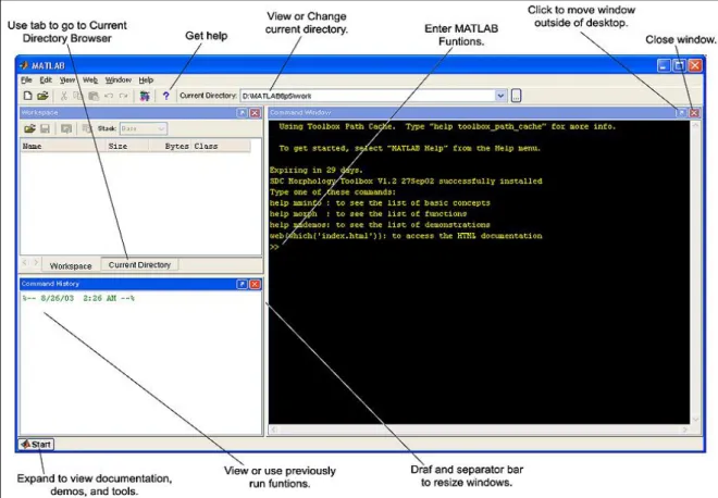
Figure 3:12 The histogram before Equalization (left) and after Equalization (right) ...43
Figure 3:13 MATLAB desktop snapshot ...44
Figure 3:14 Diagram of Image Processing Toolbox in MATLAB Program ...46
Figure 3:15 Illustration of RGB image ...47
Figure 4:1 The slide of LR 115 detector ...52
Figure 4:2 The sketch diagram of the equipments to capture image ...53
Figure 4:3 The image sample of two circles for Overlapping limitation studies ...54
Figure 4:4 Test images with circles of different diameters ...55
Figure 4:5 Test images of two ellipses with same size ...55
Figure 4:6 Test image with two squares horizontally and diagonally arranged ...55
Figure 4:7 Extraction Operations ...56
Figure 4:8 Segmentation Operations ...57
Figure 4:9 The flow chart of required data from extracted image data. ...57
Figure 4:10 The flow chart of the nuclear tracks counting simulation ...59
Figure 5:1 The Image after 1 hour radiation exposed ...61
Figure 5:2 The Image after 43 hours radiation exposed ...61
Figure 5:3 The exposed times, (a) 0 hour, (b) 1 hour. (c) 3 hours, (d) 5 hours, (e) 7 hours, (f) 10 hours, (g) 14 hours, (h) 20 hours, (i) 31 hours and (j) 43 hours ...62
Figure 5:4 Over-lapping Process of two circles with 75 pixels diameter ...63
Figure 5:5 Over-lapping Process with the objects that can still be segmented ...64
Figure 5:6 Over-lapping Process with two circles of various diameters ...65
Figure 5:7 Limitation of Segmentation based on differences of circle size (diameter) ...66
Figure 5:8 Segmentation process, diameter FO = 75 pixels and SO = 37 pixels ...66
Figure 5:9 Segmentation Process, diameter FO = 75 pixels and SO = 45 pixels ...67
Figure 5:10 Segmentation Process, diameter FO = 75 pixels and SO = 55 pixels ...67
Figure 5:11 Segmentation Process, diameter FO = 75 pixels and SO = 65 pixels ...68
Figure 5:13 Segmentation process of two ellipses ...69
Figure 5:14 Over-lapping Process of two squares diagonally arranged ...70
Figure 5:15 Segmentation Process on two squares diagonally arranged ...70
Figure 5:16 The graph of Numbers of Nuclear Track versus Exposed Time ...71
Figure 5:17 Manual Counting Method to the number of nuclear track ...72
Figure 5:18 IPTM Processing to the number of nuclear track ...72
Figure 5:19 SDC Processing to the number of nuclear track ...73
Figure 5:20 Simulated data graph after 100 times iterations ...74
Figure 5:21 Average simulated data graph ...75
Figure 5:22 Simulated data and linear extrapolation graph with the data differences ...76
Figure 5:23 Simulated data, Linear extrapolation and Nuclear track counting graph ...77
Figure 5:24 Mean area of nuclear tracks ...78
Figure 5:25 Mean area of nuclear tracks with standard deviation error bars ...79
Figure 6:1 Intersection diameter, di of the over-lapping two circles...83
Figure 6:2 Percentage difference of the nuclear tracks rate counting ...84
Figure 6:3 Standard Deviations of the area measurement ...85
Figure 6:4 The results of the nuclear track sizes based on toolboxes compared to Eghan et al. (2007) as reference (Ref.) result ...85
List of Tables
Table 5:1 Decay rate of the first object area based on the second object sizes ...68
Table 5:2 The results of counting methods ...73
Table 5:3 The results of mean area of the nuclear tracks ...79
CHAPTER 1
INTRODUCTION
1.1 Chapter Overview
Image analysis is not just important for the applications in science and engineering. It is also very significant for the clarification and understanding of the images taken by satellites, medical imaging tools such as X-ray tomography, magnetic resonance imaging (MRI) and microscopy; which involves image processing, some being much more sophisticated than others (Michielsen & Raedt, 2001). In microscope images of materials such as polymer mixtures and ceramics, the main purpose of image analysis is to provide a quantitative characterisation of the shape, structure and connectivity of the objects image. The purpose of this study is to investigate an easy-to-use and versatile method to compute the morphological properties of such images.
1.2 Research Background
Image processing is a technique to improve and enhance the raw image. There are two methods which are the Digital Image Processing and the Analog Image Processing. Digital Image Processing (DIP) is the method using computer to analyse and enhance the image (Gonzalez & Woods, 2002). It was developed at 1960s at the Massachusetts Institute of Technology, Bell Laboratories, and the University of Maryland. The processing uses image as a two-dimensional signal or input data and apply to it the standard techniques of image processing in order to get the specific output (Rosenfeld, 1969).
After three decades, the techniques of DIP have been developed by researchers in order to get the best output required. These are image representation, image
enhancement, image restoration, image analysis, image reconstruction and many more. The developments of these DIP techniques actually are based on using computer algorithms, where the noise and signal distortions can be avoided. The examples of the computer algorithm application techniques in DIP are; Feature Detection, Microscope Image Processing, Remote Sensing and Morphological Image Processing.
Image processing algorithm in Morphological Image Processing was developed based on the Mathematical Morphology (MM). MM is not just a theory but also a technique for the analysis and processing of geometrical structures, derived from the set theory, lattice theory, topology, and random functions. Generally MM is applied to digital images, and can be engaged on graphs, surface meshes, solids, and other spatial structures (Serra, 1982; Serra, 1988; Dougherty, 1992).
Image Processing Toolbox is a tool in MATLAB program. It is a set of reference-standard algorithms including MIP operator and graphical tools for image processing, analysis, visualization, and algorithm development. Application of the MATLAB program and image processing toolbox can be used in detecting an object in an image if the object has sufficient contrast from the background. As an example, the cancer cell can be detected by applying edge detection and basic morphology operations (MathWorks, 2011).
Besides Image Processing Toolbox, there is a toolbox which is known as SDC1 Morphology Toolbox for MATLAB. It is a collection Morphological Image Processing that provides morphological tools that can be applied to image segmentation, non-linear filtering, and pattern recognition and image analysis (SDC, 2011).
MIP is also used in processing nuclear track detector image. This processing is able to present granulometry and nuclear track counting results (Eghan, Buah-Bassuah, & Oppon, 2007), which is it can be used as reference in this work.
1.3 Mathematical Morphology (MM)
Mathematical Morphology is a nonlinear image processing technique that is engaged in the properties analysis of materials and material textures. It is a set of mathematical derivations that can be used as texture analysis. It has been developed almost 4 decades ago and produces many of the image processing applications. MM signifies a special method that is supported by classical linear processing. Furthermore, it improves the application of various mathematical developments of the processing and analysis of images. These areas include medical image segmentation, non-linear statistics, logic, geometry, geometrical probability, topology and various algebraic systems such as lattice and group theories. The disciplines that have been used in the classical image processing techniques normally come into view within the context of mathematical morphology, based on its development and application. There have been vast growths of interest in mathematical morphology over the past few years, which were developed by Georges Matheron (Matheron, 1975). As a result, many research approaches ranging from noise analysis to image analysis are currently being explored. Even though it was developed based on binary images, morphological applications are expanding into different fields beyond the image analysis field. For instance, lattice image processing (Maragos, 2005) and symmetry groups (Roerdink, 1993).
The application of Mathematical Morphology in image processing is a concept for operating shapes of objects in images quantitatively. All morphological methods are reduced to only two basic operations called erosion and dilation. Logical Operations also is one of the basic morphological methods (Refer to Chapter 2 for detailed information on the subject of Mathematical Morphology).
1.4 Introduction to Nuclear Track
The basics of the nuclear track operations are based on the fact that a heavy charge particle will cause extensive ionisation of the material if it passes through a medium. Some nuclear particles will be ionised along the path it takes. The path that has been made by a nuclear particle is a zone enriched area with free chemical radicals and other chemical elements. This damaged zone is the track of a nuclear, which is known as latent track (Nikezic & Yu, 2004).
If a piece of material or thin film that is sensitive to radioactivity is exposed to radioactive source for a certain period of time, the nuclear particles that passes through it will ionise the film and create the latent track. Theoretically, the number of this nuclear latent track produced from a radioactive source is proportional to time. However, the thin film containing latent tracks needs to be exposed to some chemically aggressive solution, where chemical reaction will occur extensively along the latent tracks. This chemical solution is required to form the ‘track’ of the particle, which may be seen under an optical microscope. This procedure is known as detector etching or track visualization.
The thin film that is used in the nuclear track processing is called track detector. They are three common types of track detectors that are used in nuclear track. They are CR-39 detector which is based on polyallyldiglycol carbonate, cellulose nitrate, and the well-known LR 115, which will be used in these studies.
In order to continue with the track analysis and image processing procedure, the nuclear track detector requires conversion to an image. As an image, granulometry analysis and nuclear tracks counting can be succeeded (Eghan, Buah-Bassuah, & Oppon, 2007).
1.5 Motivation
We know there are many image processing problems that can be solved using certain techniques, which is suitable with their problems characteristic. We also know that image processing can be run or processed using many types of software. For that reason, the main motivation for conducting this research is to find out the capability of the combination between MATLAB program and also a MATLAB toolbox developed by third party (SDC Morphology Toolbox) in processing the images.
There are various problems in the field of image processing, which can be solved through certain techniques and algorithms based on the types of problems. Based on this known problems, we would like to apply an image processing method known as the Morphological Image Processing in order to find more efficient approaches or techniques to deal with the problems. In addition, the SDC Morphology Toolbox was built based on Morphological Image Processing principle.
1.6 The Purpose and Objective of the Research
The main goal of this research is to study Morphology Image Processing (MIP) and its application to nuclear track images by comparing the results obtained from using Image Processing toolbox and SDC Morphology toolbox application. This thesis has the following objectives;
i. To study the capability of SDC Morphology Toolbox as a morphology image processing tool in conjunction with the MATLAB platform, regardless whether the image is real or artificial (Pritchard, 2002; Marshall, 1992; Quadrades & Sacristán, 2001).
ii. To use these toolboxes to perform dot counting (nuclear track counting) profile at arbitrarily set areas and compare with result from simple particle (nuclear track) counting simulation. We also use these toolboxes to perform granulometry (area
measurement) to obtain the average of the mean area profile of exposed nuclear track over various exposure times and thus obtain the diameter of the mean area. iii. To study how the toolboxes perform nuclear track counting on images of nuclear
tracks in which some of the tracks are over-lapping with each other. We then separate the over-lapping tracks based on how much the objects overlap and with different object shapes to obtain the segmentation limit value.
iv. To compare the SDC Morphology Toolbox and the Image Processing Toolbox and determine which toolbox gives the more precise and accurate nuclear track counting and granulometry (area measurement).
1.7 Chapters Overview
This dissertation contains five main chapters. The overview of each chapter is given below.
First Chapter
This is the introduction chapter with discussion on research background, mathematical morphology, nuclear tracks, motivations of the research and purpose and objective research.
Second Chapter
In this chapter theoretical background of Image Processing and Mathematical Morphology are discussed and explained including the algorithms, which are relevant to the objectives of the research. A section related to Mathematical Morphology will give some ideas on what MIP is all about. Then the chapter included a brief of theory discussion of object extraction, granulometry and nuclear track formation.
Third Chapter
The descriptions, that focuses on MATLAB as a programming platform for Image Processing including Image Processing Toolbox and SDC Morphology Toolbox.
Fourth Chapter
The chapter is all about research methodology.
Fifth Chapter
All of the research findings and the discussions relating to the result obtained are found in this chapter.
Sixth Chapter
This section provides the final conclusions and further deductions, specifically from the research findings.
CHAPTER 2
THEORY AND BACKGROUND
2.1 Chapter Overview
In this chapter, theoretical background of image processing and mathematical morphology, including the relevant algorithms are discussed. The basic concepts used in the SDC Morphology Toolbox for MATLAB are also covered.
2.2 Theoretical Background of Image Processing
There are many possible definitions for the term of Image Processing and Computer Vision. The most common one that will be stated in this thesis is that image processing aims to process an image, usually by a computer to produce informative image output. On the other hand, computer vision processes the image and produces it into some form of generalised information about the image, such as labelled regions. Ballard and Brown (1982) came out with the statement that “Computer Vision is the
enterprise of automating and integrating a wide range of processes and representations for visual perception”. They also include the term of image processing within this
definition by implying that image processing is one of the many steps in computer vision. Niblack (1986) describes image processing as “the computer processing of
pictures”, whereas Computer Vision includes many techniques from image processing,
but is broader in the sense that it is concerned with a complete system.
In many situations, image processing is operated with taking an array of pixels (image) as input and constructing a new array of pixels as output which somehow represents an improvement and enhancement to the original array. Image processing methods have been divided into Real Space methods and Fourier Space methods. The
Real Space methods are engaged in processing the input pixel array such as Grey Level Thresholding, Image Smoothing, and Detection of Points, Lines and Edges. The Fourier Space methods work by deriving a new representation of the input data by performing a
Fourier Transform, which is then processed. Finally, an Inverse Fourier Transform is
performed on the resulting data to give the final output image.
A digital image can be written down as a[m, n], which ‘a’ is matrix with m rows and n columns, and also represented in a 2-D discrete space. It is derived from an analogue image a(x, y) in a 2-D continuous space through a sampling process, also known as digitisation. The process will digitise the image function, f(x, y) spatially and in amplitude (Russ, 2008).
The digitisation process of an image is shown in Figure 2:1, which the analogue image or 2-D continuous image can be presented as a(x, y) and divided into N rows and
M columns. The intersections point of a row and a column is known as pixel. The value
assigned to the integer coordinates of a pixel [m, n] with {m = 0, 1, 2, ..., M-1} and {n = 0, 1, 2, ..., N-1} is a[m, n]. In many cases, the 2-D continuous image a(x, y) which is considered to be the physical signal that gives limit effect on the face of a 2-D sensor, where the signal is an actual function of variables together with depth (z), colour (λ), and time (t). In this study, the images are 2-D, monochromatic and static images.
Figure 2:1 Digitisation of a continuous image. The pixel at coordinates [m = 7, n = 3] has the integer brightness value 212.
The image shown in Figure 2:1 has been divided into pixels of N = 22 rows and
M = 15 columns. A value assigned to each pixel is the average brightness of the pixel
rounded to the nearest integer value. The process of representing the amplitude of the 2 dimensional signals, at a given coordinate as an integer value with different grey levels is usually referred to as amplitude quantization or simply quantization.
2.3 Mathematical Morphology Theoretical Background (The Concepts of Mathematical Morphology)
One of the abilities of image processing and analysis refers to geometrical concepts such as size, shape, and orientation. Mathematical morphology uses concepts from set theory, geometry and topology to analyse geometrical structures in an image (Heijmans, 1994). The name Mathematical Morphology (MM) was introduced in 1966 (Serra & Soille, 1994) and the theoretical treatment presented by Matheron (1975) and Serra (1982; 1988). MM provides an approach to image processing, which is based on
Rows
Columns
, , , ,
methodology, designed for the analysis of the geometrical structure in an image. The method has also found applications in several other fields, such as medical diagnostics, histology, industrial inspection, computer vision, and character recognition (Kukielka & Woznicki, 2001).
MM examines the shapes or geometrical structure of an image by probing it with small patterned images which is called structuring elements. These structuring elements can take in various shape and size. A non-linear image will be produced from this procedure, which is suitable for studying geometrical and topological structures. These MM operators are then applied to an image in order to make certain features perceptible and apparent. The process of reducing the object shape in the image to a sort of caricature (skeletonization) will distinguish the meaningful information from inappropriate distortions. For example, the shape of an object can be transformed to the digital image of a symbol by reducing each connected component to a one pixel thick skeleton while retaining the symbol’s object shape. The effectiveness of this skeletonisation process is sufficient for recognition and it can be handled much more economically than the full symbol.
Theoretically, mathematical morphology studies operators between complete lattices, specifically nonempty sets equipped with a partial order relationship for which every subset has an infimum and a supremum. Appendix 2A gives further details about infimum and supremum. In fact, MM was developed from translation invariant operator between complete lattices and it can be represented by means of elementary morphological operators. An image operator can be created by composing elementary morphological operators. However, this approach is not practical when a large number of elementary operators are used. Fortunately, most applications can be successfully operated within below the limited reasonable number of morphological operators.
Therefore, an image analysts need to identify the category of morphological operators for a particular problem, whether it is for shape detection, extraction, or filtering.
Morphological operations tend to simplify, enhance, extract or describe image data. Figure 2:2 shows the relationships among the basic elements of MM.
Figure 2:2 A mathematical tools diagram that studies operators on complete lattices.
Morphology originally comes from a branch of biology that refers to the form and structure of animals and plants. Also, it is used for the study of geometry and topology of patterns. In addition, integral-geometry Morphological Image Analysis (MIA for short) employs additive image functionals to assign numbers to the shape and connectivity of patterns formed by the pixels in the image. A part from that, integral geometry provides the precise mathematical framework to define these image functionals (Santaló, 2004; Stoyan, Kendall, & Mecke, 1996; Michielsen & Raedt, 2001). The fundamental theorem of integral geometry states that under certain conditions, the number of different additive image functionals is equal to the dimension of the pattern plus one (SDC, 2011). Thus, in the case of a 2-D image, there are exactly three of these functionals, called quermassintegrals or Minkowski functionals. For a
Mathematical Morphology Algebra Complete lattices Operators Erosion-Dilation Topology Hit or Miss Geometry Convexity – Connectivity Distance Applications
second step is to study the behaviour of the three or four numbers as a function of some control parameters, such as time, density, and so on (Michielsen & Raedt, 2001).
A significant feature of MIA is the massive contrast between the simplicity of implementation or use and the level of sophistication of the mathematical theory. Without a doubt, as follows, the calculation of the image functionals merely amounts to the proper counting of, for example faces, edges and vertices of pixels. The application of MIA requires little computational effort. Another appealing feature of MIA is that the image functionals have a geometrically and topologically intuitive and hence, also have perceptually clear interpretation for 2-D images as they correspond to the area, boundary length, and connectivity number. The four functionals for 3D images are the volume, surface area, integral mean curvature and connectivity number (Michielsen & Raedt, 2001).
2.3.1 Morphological Image Processing
Basically, the digital form image can be produced as an output from any image processing program (software), which the MATLAB itself could be used as a digitised image generator software. The digitised images are free of noise and other artifacts that may affect the geometry and topology of the image structures or area of interest. Such perfect images are easily generated by a computer and are very useful for the development of theoretical concepts and models. Unfortunately, genuine pictures or patterns obtained from computer simulations are usually imperfect. Therefore, some special form of image processing may be necessary before attempting to make measure-ments of the features in the image (Michielsen & Raedt, 2001).
In Morphological Image Analysis, it is very important to acquire the geometric and topological content of the image from the operations that are used to enhance the image quality. The morphological image processing (MIP) technique will be reviewed
in the following section and is well adapted for this purpose. This is because MIP and MIA are based on the same mathematical concepts. Most importantly, it is very flexible, fast and easy to use. Pioneering work in this field was carried out by Matheron (1975) and Serra (1982).
The most important reason why we use mathematical morphology as the main principle in solving various Image Processing problems in this research is because it is a special mathematical tool or method for investigating geometric structure in binary and also greyscale images. In other words, mathematical morphology is not just a theory of geometric, but it also known as a geometric approach to Image Processing and Analysis. By using this approach, it makes the images become easier (becoming noiseless) to analyse. This is what we need in this research where the visual perception requires transformation of images so as to make particular shape information observable. The goal of this approach is to distinguish meaningful shape or structure information from irrelevant one (images). The vast majority of shape processing and analysis techniques are based on designing a shape operator which satisfies desirable properties. Figure 2:3 and Figure 2:4 are shown below to display the difference between greyscale images and binary images. The binary images only show white and black colour, which the pixel values only give ‘0’ and ‘1’ as discussed earlier.
(a)
(b) Figure 2:3 Greyscale images
(a)
(b) Figure 2:4 Binary Images
Image analysis consists of obtaining measurement characteristics to images under consideration. For example, geometric measurements determine object location, orientation, area, and length of perimeter.
The basic operations associated with an object are the standard set operations
union {}, intersection {}, and complement {C} and also translation, which is given by a vector x and a set A. The translation, A + x, is defined as equation 2:1 below;
2:1
Since we are dealing with a digital image composed of pixels at integer coordinate positions (Z2), thus implies restrictions on the allowable translation vectors x.
The basic Minkowski set operations addition and subtraction can now be defined. The individual elements that comprise of B are not only pixels but also vectors, as they have a clear coordinate position with respect to [0, 0]. Given two sets equation A and B, as stated below;
Minkowski addition:
2.3.2 Hit-or-Miss Transformation (HMT)
The language of MM is that of a set theory, where the set represents binary and grey level images. For instance, the set of all white pixels in a black and white image form a complete description of the image and can also be regarded as an image object. MM extracts information about the geometrical structure of an object by transforming it through its interaction with another object, called the structuring element, which is of simpler shape than the original object. The information about size, spatial distribution, shape, connectivity, convexity, smoothness, and orientation can be obtained by transforming the image object using different structuring elements. An example of a structuring element, B centred at a point x is given in Figure 2:5. The point x can be x
seen as the origin of a coordinate system, which permits to address any of the positions of B by a vector b. x
Figure 2:5 Example of a (non-symmetric) structuring element, centered at x. The vector
b permits to address different positions.
The most fundamental operator for shape detection is known as Hit or Miss
Transformation (HMT) (Serra, 1982). It is a point by point transformation of a set X.
Structuring element, B is composed from two sub-sets, x 1
x
B and Bx2 which is centred at the same point x, as follows;
2:2
The set 1
x
B only contains ones and the set 0
x
B only contains zeros. Both sets may contain points of indifferent values, which means one or zero. Apart from that, point x
1 1 1 1 1 1 1 1 1 1 1 1 1 1 1 1 1 1 1 1 1 1 1 1 1 1 1 1 1 1 1 1 1 1 1 1 1 1 x 1 1 1 1 1 1 1 1 1 1 1 1 1 1 1 1 1 1 1 1 1 1 1 1 1 1 1 1 1 1 1 1 1 1 1 1 1 1 1 1 1 1 1 1 1 1 1 1 x 1 1 1 1 1 1 1 1 1 1 b
belongs to the HMT, XBof X, if and only if B1x is included in X and Bx0 is included in the complement of X, as follows;
2:3
An illustrative example for an image on a discrete grid is given in Figure 2:6. The structuring element is 1 at its centre and 0 on the right side, and thus B1x is one at the centre and of indifferent value on the right (represented by a point in Figure 2:6). Whereas Bx0 is of indifferent value at the centre and zero on the right side. It is easy to observe that only the right border points result from the HMT transformation. The sample structuring element shown below (Figure 2:6) is taken from the online documentation of SDC Morphology Toolbox, which re-groups a number of structuring elements B and is also interesting for various image analysing tasks.
0 1 0
HMT 1 0 0 0 1 .
1 1 0 0 0 0 1 1 .
0 0 0 0 0 0 . . 1
Figure 2:6 Example of a HMT transformation
2.3.3 Erosion
Erosion reduces the size of an object and eliminates features that are less than the scale of the neighbourhood as defined by the structuring element. It can be obtained by applying the HMT where Bx0 is the empty set. Hence, the eroded set Y of X are the
locus of the centres x of 1
x
B included in the set X. It can also be obtained by the classical Minkowski subtraction (Haralick & Shapiro, 1991), , where X is b
the translated version of X by the vector b. Erosion is thus defined as (Serra, 1982);
From the definition
b B
b
B is the transposed set of B, where the reflected set of B is with respect to the origin, and 1,B is the erosion of X by B of size 1. This process is viewed as a removing process of a certain number layers of the object. An example of erosion is given in Figure 2:7 and Figure 2:9.
X
Figure 2:7 Minkowski subtraction is
2.3.4 Dilation
Dilation expands the size of objects on the scale of structuring element neighbourhood. It is the dual operation of the erosion with respect to complementation, meaning a dilation of is equal to an erosion of X. It is the locus of the centres of the
1
x
B which hit the set X. Dilation can also be expressed in terms of Minkowski addition and is defined as follows (Serra, 1982):
2:5
Consequently, the transposed set B is occupied to be able to make the analogy with the HMT. An example of dilation is given in Figure 2:8, where the process can be seen as the addition of layers to the object. See Figure 2:9 for more examples of dilation processes using MATLAB.
X
Figure 2:8 Binary Morphological Dilation process
(a) Original Image
(b) Structuring Element
(c) Erosion image, B( )X (d) Dilation Image, B( )X
Figure 2:9 Example of erosion and dilation of a binary set X
2.4 SDC Morphology Toolbox for MATLAB
The SDC Morphology Toolbox for MATLAB is an accumulation of greyscale morphological tools that can be applied to image segmentation, non-linear filtering, pattern recognition, and image analysis (SDC, 2011). It includes effective segmentation functions such as watershed and connected filters based on reconstruction. The SDC
to many real life image processing problems. For instance, several images in the field of machine vision, medical imaging, desktop publishing, document processing, food industry, agriculture, and so on, are included in the toolbox.
The SDC Morphology Toolbox is a set of functions or programs for Image and Signal Processing. The functions in this toolbox are based on the theory of Mathematical Morphology, which have been discussed in section 2.3. It is a non-linear approach for the representation of image and signal transformation, which makes it practical for analysing some Image and Signal Processing problems generally, such as segmentation, and extraction of quantitative information, noise reduction and compression. Mathematical Morphology has a special characteristic which allows us to learn generic transformations of discrete signals directly, without appealing to continuous approximations. This characteristic allows for the development of efficient algorithms of compact integer data structures.
Nowadays, researchers in image processing and computer vision field are increasingly recognising that simple algorithms derived from mathematical morphology can be extremely useful in all kinds of applications. Hence, MATLAB is becoming increasingly important as the programming environment for image processing. Furthermore, the addition of the MORPHOLOGY TOOLBOX for MATLAB enhances MATLAB image processing capabilities.
2.4.1 Availability of the Toolbox
The SDC Morphology Toolbox is generated mostly using automatic methods. This ensures that the syntax and conventions used are very consistent with the toolbox. The images loaded in SDC Morphology Toolbox are represented as 1-D, 2-D, or 3D arrays, with pixels of types uint8, uint16, and logical uint8 (binary). The image data type in uint8 represents positive integers from 0 to 255, the uint16 image data type
represents integers from 0 to 65535, and the logical uint8 represents just the numbers 0 and 1. Structuring elements and a sub-image are needed to process the image.
The toolbox has Interval functions which are also known as hit-or-miss
templates. They are useful to process the morphological images. Generally, these
functions are the functions that create interval to detect end-points of curves, and interval for homotopic thickening and thinning of binary image. The toolbox also has a few functions that can be applied to manipulate the interval, whether to rotate by an angle or to visualize it. This Interval function also has unique functions that are capable to create hit-or-miss template or an interval itself, based on a pair of structuring elements. For more details about Interval functions, please see its example in Appendix 2B.
2.4.2 General rules
The SDC Morphology toolbox has several general rules which we need to comprehend before applying it. These general rules make it easier for us to understand and handle the toolbox.
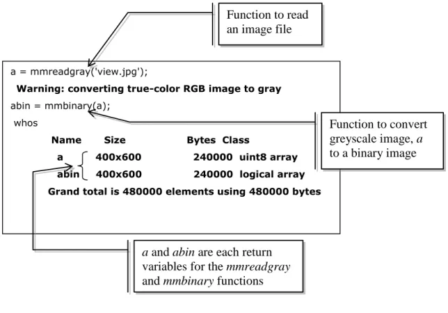
The first rule stated that each function of the toolbox can return only one variable, for example; the application of mmreadgray and mmbinary functions in the box below will return each, a variable of ‘a’ and ‘abin’, which are the images. Figure 2:10 shows the MATLAB script, which the functions return one variable each.
Figure 2:10 The MATLAB script of the functions that returns one variable each
In addition, the command line of MATLAB can be engaged from left to right, and the SDC Morphology toolbox’s operands can also be optional from left to right only. Mmconv is one of the functions in SDC Morphology Toolbox. Please refer to Appendix 2C for more detailed information regarding conventions that are used in the SDC Morphology Toolbox.
The toolbox default parameter of the structuring element is mmsecross, which is the elementary 33 cross. The mmsecross function generates the structuring element B, formed by r successive Minkowski additions of the elementary cross. In other words, the 33 cross centred is at the origin with itself. If r = 0, B is the unitary set that
contains the origin. If r = 1, B is the elementary that cross itself. Equation 2:6 below which proves how the mmsecross functions;
2:6
a = mmreadgray('view.jpg');
Warning: converting true-color RGB image to gray
abin = mmbinary(a); whos
Name Size Bytes Class
a 400x600 240000 uint8 array abin 400x600 240000 logical array Grand total is 480000 elements using 480000 bytes
a and abin are each return
variables for the mmreadgray and mmbinary functions
Function to read an image file
Function to convert greyscale image, a to a binary image
And then, Figure 2:11 demonstrates the MATLAB script to demonstrate the function of mmsecross. se1 = mmsecross; mmseshow(se1) ans = 0 1 0 1 1 1 0 1 0 se2 = mmsecross(2); mmseshow(se2) ans = 0 0 1 0 0 0 1 1 1 0 1 1 1 1 1 0 1 1 1 0 0 0 1 0 0
Figure 2:11 The MATLAB Script of mmsecross function
In other words, the radius, r needs to be determined to mmsecross in order to create the structuring elements with the radius more than 1.
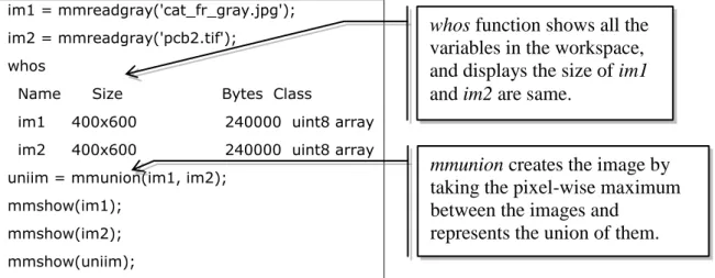
All the images in most functions must have the same data type and size. This rule states that the data type and size of images should be in the same value in order to make the functions of SDC Morphology Toolbox run smoothly. This can be seen below in the example of MATLAB script with regard to this matter.
im1 = mmreadgray('cat_fr_gray.jpg'); im2 = mmreadgray('pcb2.tif');
whos
Name Size Bytes Class
im1 400x600 240000 uint8 array im2 400x600 240000 uint8 array uniim = mmunion(im1, im2);
mmshow(im1); mmshow(im2); mmshow(uniim);
Figure 2:12 The MATLAB Script that shows data type and size are in the same value The default structuring
element created by
mmsecross (r = 1)
Structuring element by r = 2 Function to display
structuring as an image
whos function shows all the
variables in the workspace, and displays the size of im1 and im2 are same.
mmunion creates the image by
taking the pixel-wise maximum between the images and
Figure 2:13 Image, im1 Figure 2:14 Image, im2
Figure 2:15 Final image, uniim
As the result of the script which finally produces three images. This can be seen in Figure 2:13, which shows the first image from the script, and then Figure 2:14, which shows the second image, and the final image in Figure 2:15 represents their union image.
The toolbox has the capability to operate an image with a constant value. This constant is regarded as a constant image and is the same size as the other images. This can be applied to mmunion function where the image besides the first images could be a constant (SDC, 2011), Refer to Appendix 2D for more detail about mmunion function.
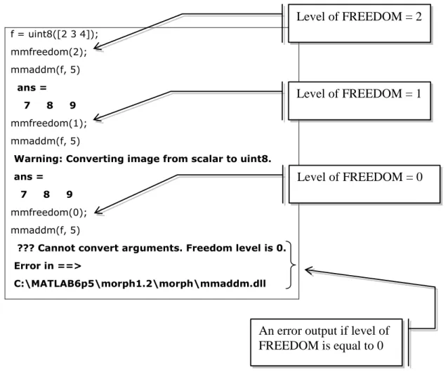
Furthermore, inside the SDC Morphology Toolbox, there is a function called
mmfreedom, which controls the automatic data type conversions. There are 3 possible
levels, called FREEDOM levels (SDC, 2011). In this research, we use type conversion ‘1’. The FREEDOM levels are set or inquired by mmfreedom function.
Figure 2:16 MATLAB FREEDOM levels script
Figure 2:16 shows the result of the MATLAB script, the level of FREEDOM that is equal to ‘1’ is more appropriate in applying the toolbox because the user will realize to what is actually happening to the programming script and the variables, especially when the warning sign appear after the image type conversion is completed.
2.5 Objects Extraction Review
This sub-topic is about reviewing theoretically the extraction of the objects from the image. Firstly, the operator that is always used as a first step to start the script in this research is called Opening operator. Then, the derivation from the erosion operation occurs followed by a dilation operation (Pratt, 2001). A part from that, there are a few functions of this operator that will always make the objects in the image smooth.
f = uint8([2 3 4]); mmfreedom(2); mmaddm(f, 5) ans = 7 8 9 mmfreedom(1); mmaddm(f, 5)
Warning: Converting image from scalar to uint8.
ans = 7 8 9
mmfreedom(0); mmaddm(f, 5)
??? Cannot convert arguments. Freedom level is 0. Error in ==>
C:\MATLAB6p5\morph1.2\morph\mmaddm.dll
Level of FREEDOM = 1
Level of FREEDOM = 0 Level of FREEDOM = 2
An error output if level of FREEDOM is equal to 0
Concurrently, the small images or islands will be eliminated depending on the structuring elements condition and they will also divide the narrow connection (Gatos & Perantonis, 2004). Object extraction can also be improved as fast opening functions to granulometries applications (Vincent, 1993; Vincent, 1994a). Figure 2:17, Figure 2:18 and Figure 2:19 illustrate the example of the Opening operator application using disk shape structuring element to the artificial (synthetic greyscale) image.
Figure 2:17 Original image Figure 2:18 The image after Opening operation
Figure 2:19 The overlay of original and open image
Hence, after the Opening operation has been done to the research image, the next process that follows is image reconstruction, which is also known as Infinite Reconstruction (Serra, 1983). Infinite Reconstruction (inf-reconstruction) constructs or rebuilds the portion of interest in the image by means of image filtering, ‘top-hat’, segmentation, etc. (Vincent, 1993; Heijmans, 1994). In other words, the purpose of the process is to give back the required objects into the image. The following figures
image, where Figure 2:20 shows the original image, Figure 2:21 shows the image after erosion processing and Figure 2:22 shows a reconstructed image.
Figure 2:20 Original image Figure 2:21 Eroded Image
Figure 2:22 Reconstructed image
The following step is to subtract the research image in order to obtain a subtracted image based on the reconstructed image, where the portion of interest is more significant with the background pixel value uniformly (Serra, 1983; Gonzalez & Woods, 2002). See Figure 2:23, Figure 2:24 and Figure 2:25 that illustrate the example of subtraction operation for the sample image taken from SDC Information System’s site. Besides that, the operation of image comparison would be useful in order to obtain the image with uniformly pixel value background (SDC, 2011).
Figure 2:23 First image Figure 2:24 Second image
Figure 2:25 Subtracted image
After a few operations have been done to the image, the Area Opening operation will be proposed in this research where the grains (unwanted objects) will be removed and only the required objects or shapes will be kept (Haralick, Sternberg, & Zhuang, 1987; Scott & Mukherjee, 2000). The Area Opening operation will remain the portion of interest based on the conditions given, for example, in choosing the area of the object pixel wisely (SDC, 2011).
In addition, Close Holes operator can be also used in order to get fine extracted objects in the image. Close Holes is one of the morphological operators that function as closing the holes of the image or filling the holes in every connected component of an image. It is also resulted from the improvement of the closing operator. This is very useful for granulometry function analysis of the size of the objects in the image because it will entirely produce the shape of objects in the image without changing their contour (Ruberto & Dempster, 2000). Figure 2:26 below shows the flow chart of the basic and complete object extracting processes as have been discussed above.
Figure 2:26 Object extracting process Flow Chart
2.6 Over-lapping Objects Extraction Review
This review is extended from the previous review (Section 2.5), which is about extracting the over-lapping objects from the image. There are certain processes for this review that are similar with the subject-matter discussed above, and the processes include thresholding, marking, and Geodesic ‘Skeleton by Influence Zones’ (SKIZ) which will be discussed later.
Generally, thresholding is a segmentation process of the objects in the image from the rest of image area and this process produces segmented objects, which we can distinguish from the other areas (Gonzalez & Woods, 2002). In order to get smooth segmented objects, an opening process is required for the image. Consequently, the distance transformation (Shih & Mitchell, 1992) and dilation operation can be applied to these segmented objects in order to obtain marked objects.
Sample Image (greyscale or binary) Opening process Image reconstruction Subtraction opening Image Comparison Area Opening Operation Additional process: Close holes operation
Extracted image
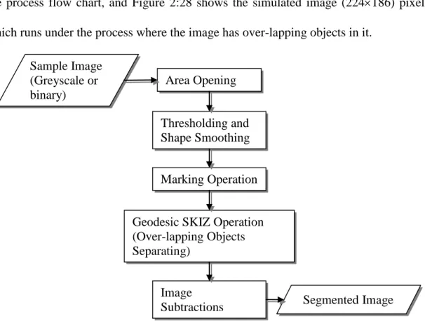
As stated above, this section is about extracting the over-lapping objects from the image. The separation of the over-lapping objects can be done by Geodesic SKIZ Approach (Vincent & Dougherty, 1994), a process which has a watershed operation. The process of watershed is based and limited by the markers image and applied to the negated distance function image. Furthermore, to get fully objects separation, a subtraction process can be applied to the Geodesic SKIZ processed image of the segmented image. This operation will separate the objects. See Figure 2:27 that shows the process flow chart, and Figure 2:28 shows the simulated image (224186) pixels, which runs under the process where the image has over-lapping objects in it.
Figure 2:27 Over-lapping objects separating process Sample Image (Greyscale or binary) Area Opening Thresholding and Shape Smoothing Marking Operation
Geodesic SKIZ Operation (Over-lapping Objects Separating)
Image
(a) (b)
(c) (d)
Figure 2:28 Images of Over-lapping extraction process; (a) Original image, (b) Thresholded image, (c) Image after Geodesic SKIZ process, and
(d) Over-lapping objects segmented image
2.7 Measurement of the Objects/Grains, (Granulometry)
The objects that have been extracted and segmented as previously discussed can be used for measurement analysis, which is also known as Granulometry Analysis (Vincent, 1994b). Granulometries are programmed sets of morphological openings and closings operator that can be applied as detail image removals depending on its structuring elements’ size and characteristic. Because of this reason, it becomes one of our tasks in this research to discover the toolbox capabilities’ on Granulometries. Based on the SDC Morphology Toolbox’s demonstrations and documentations as our references, we need to perform some Granulometries tasks to our images that have been extracted and segmented (the objects) as above. For other references on recent granulometry research, please refer to Ves, Benavent, Ayala, & Domingo (2006).
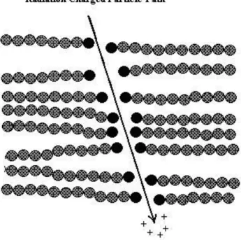
2.8 Nuclear Track Formation Mechanism and Its Shape
The formation of the nuclear track could occur when the radiation particle penetrated the film detector (nuclear track detector). The detectors are basically insulated by electrically solid materials where the passage of heavily charged particles creates trails along their paths and these damage zones on an atomic scale are called latent tracks. The treatment to these latent tracks using chemical or electrochemical etching allows their visualisation under optical microscopes.
When the detectors are exposed to the radiation source, the ionising particle interacts with matter and transfers a part of its energy to the electrons of the medium with some rate of energy loss. When the energy loss is above a certain critical value, local structure transformations or etched track are formed. These transformations in the case of polymers can be explained by splits in the molecular chains and formations of new components chemically very reactive along the particle trajectory. Typically the latent track formed has diameters from 1 to 10 nm (Fleischer, Price, & Walker, 1975). Figure 2:29 gives a schematic illustration of the effect caused by the passage of charged particles. Figure 2:30 shows a schematic of the film detector with latent track before and after the etching process.
Figure 2:29 The schematic illustration of effect caused by the passage of charged particle
Figure 2:30 The schematic of the film detector with latent track before and after the etching process
The shapes of the nuclear tracks were not always regularly circular (circle) when viewed from above, there can also be oval in shape (ellipse), this depends upon the angle of incidence on the detector surface. Larger incidence angles will make nuclear track’s shape more elliptical (oval) (Khan & Khan, 1989), see Figure 2:31. Some
view of image of a single-crystal mica template formed by nuclear track etching (Sun & Hao, 2005), see Figure 2:32.
Figure 2:31 The top view of nuclear tracks ellipse shape (Khan & Khan, 1989)
Figure 2:32 The top view of nuclear tracks diamond shape (Sun & Hao, 2005)
2.9 Chapter Summary
The effect of these MIP operations with their characteristics of structuring elements to the images could produce a variety of results depending on the parameters of structuring elements. The MIP has two important basic operators, namely the Erosion and Dilation, which could expand the procedure of the MIP. For instance, there are the Opening and Closing operations. The MIP that has a built-in SDC Morphology Toolbox is a complete tool of MIP applications, along with the MATLAB system.
There are 3 processing procedures that will be used with regard to this research; they are Object Extraction, Over-lapping Objects Extraction and Granulometry. All of them are related to MIP. It means that these procedures will also be utilised to test SDC Morphology toolbox and Image Processing toolbox capabilities.
CHAPTER 3
THE MATLAB TOOLBOX FOR IMAGE PROCESSING
3.1 MATLAB Image Processing
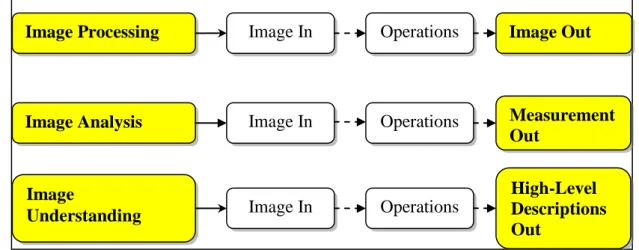
Fundamentally, image processing is basically to perform operation on images. In general terms, image processing refers to the manipulation and analysis of two dimensional visual images. It is any operation that acts to improve, correct, analyse, or change an image in some ways to produce better images as the objective requires (Forsyth & Ponce, 2003; Horn, 1986; Jain, Kasturi, & Schunck, 1995). Figure 3:1 shows the differences between image processing, image analysis and image understanding.
Figure 3:1 Three manipulations of image
Image processing operations can be generally divided into three major categories. They are image compression, image enhancement and restoration, and measurement extraction. Image compression involves reducing the amount of memory needed to represent a digital image (Matheron, 1988; User's Guide, 2001; Using MATLAB, 1999). The purpose is to compress the size of a file (picture or image)
Image Processing Image Understanding Image Analysis Image In Image In Image In Operations Operations Operations Image Out Measurement Out High-Level Descriptions Out
without reducing the quality of the picture or image itself. For instance, Joint Photographic Experts Group (JPEG) is one of the most popular and comprehensive continuous tone (as opposed to binary), still frame compression standard format. Further information related to image compression, other images or graphics file format and JPEG 2000 can be found in Gonzalez and Woods (2002), and Miano (1999).
A digital image can be composed (consists) of a set of points which may be defined as a two-dimensional function, f(x, y); where x and y are spatial (plane) coordinates, and the amplitude of f at any pair of coordinates (x, y) has its own brightness which is called the intensity or grey level of the image at that point, see Figure 3:2. These points are called ‘pixels’ (pixel stand for picture element). The number of pixels within a unit length divided by area is called ‘resolution’, the level of detail measured in units per inch.
Figure 3:2 Pixels
Various operations may be performed on the pixels of the original image to produce a new image. These operations may be performed on each pixel in isolation or relative to other pixels in the image (Matheron, 1975). The purpose of these operations is to improve the visual appearance of images, or to prepare images for the
may be used to clean up an image by removing the noise (noise reduction), improve the contrast of the image and highlight elements with certain characteristics. It may also overcome distortions such as blurring or warping of an image caused by a camera or scanner, and then compensate for uneven illumination which existed in the image.
The basic of image processing operations may also be carried out by filtering or mask processing operation, which attempts to highlight significant features and suppresses insignificant detail based on some neighbourhood operations. This is done by working with the values of the image pixels in the neighbourhood and the corresponding values of a sub-image (filter, mask, kernel, template, or window) that has the same dimensions as the neighbourhood.
Edge detectors operation (detecting the edge of the objects in the image) highlights the significant transitions of the object in the image. This will specify the boundaries within the image. Edges are places in the image with strong intensity contrast. Since edges often occur at image locations representing object boundaries, edge detection is extensively used in image segmentation when we want to divide the image into areas corresponding to different objects. Representing an image by its edges has the further advantage that the amount of data is reduced significantly while retaining most of the image information. Since edges consist of mainly high frequencies, theoretically, edge detection can be done by applying a high-pass frequency filter in the Fourier domain or by convolving the image with an appropriate kernel in the spatial domain. Practically, edge detection is performed based on spatial domain, is more computational and gives better results. Figure 3:3, Figure 3:4 and Figure 3:5 show the differences of Saturn edge detected images using Sobel and Canny operators. This processing procedure was produced by using MATLAB script, see Appendix 3A.
Figure 3:3 Original image of Saturn.
Figure 3:4 Edge detection by Sobel operator.
Figure 3:5 Edge detection by Canny operator.
Texture analysis involves identifying variation in brightness from one pixel to the next or within a small region in the image. Then, it can be defined as the pattern of