LAPORAN AKHIR PENELITIAN PASCASARJANA DANA ITS 2020

LAPORAN AKHIR

PENELITIAN PASCASARJANA

DANA ITS 2020

(

Studi Pola Arus Geostopik di Perairan Indonesia menggunakan Data

Satelit Altimetri Jason-2 dan Jason-3)

Tim Peneliti :

Dr. Eko Yuli Handoko, ST. MT. (Teknik Geomatika/FTSPK)

Danar Guruh Pratomo, ST., MT., PhD (Teknik Geomatika/FTSPK)

Mokhamad Nurcahyadi, ST, M. Sc, Ph.D/ (Teknik Geomatika/FTSPK)

Fajar Kharisma, ST. (Teknik Geomatika/FTSPK)

Desi Suci Richasari (Teknik Geomatika/FTSPK)

DIREKTORAT RISET DAN PENGABDIAN KEPADA MASYARAKAT

INSTITUT TEKNOLOGI SEPULUH NOPEMBER

SURABAYA

Daftar Isi

Daftar Isi ... i

Daftar Tabel ... ii

Daftar Gambar ... iii

Daftar Lampiran ... iv

BAB I RINGKASAN ... 2

1.1

Latar Belakang ... 2

1.2

Perumusan Masalah dan Tujuan Penelitian ... 4

1.3

Manfaat dan Urgensi Penelitian ... 4

BAB II HASIL PENELITIAN ... 2

2.1

Pengecekkan Data RADS ... 2

2.2

Perhitungan SSH dan SLA ... 2

2.3

Rata-rata SLA per cycle ... 4

2.4

Intercalibrated Tandem Mission... 4

2.5

Gridding ... 6

2.6

Perhitungan Arus ... 6

BAB III STATUS LUARAN ... 8

BAB IV KENDALA PELAKSANAAN PENELITIAN ... 9

BAB V RENCANA TAHAPAN SELANJUTNYA ... 10

BAB VI DAFTAR PUSTAKA ... 11

BAB VII LAMPIRAN ... 12

Daftar Tabel

Daftar Gambar

Gambar 2.1. Pengecekan Data RADS

2

Gambar 2.2. Script Pembacaan Data .nc

3

Gambar 2.3. Script Perhitungan SSH

3

Gambar 2.4 Script Perhitungan SLA

3

Gambar 2.5. Hasil Perhitungan SSH dan SLA

4

Gambar 2.6. Script Perhitungan Rata-rata SLA

4

Gambar 2.7. Grafik Time Series SLA sebelum Interkalibrasi

4

Gambar 2.8. Grafik SLA Terinterkalibrasi

5

Gambar 2.9. Grafik Time Series SLA Sesudah Interkalibrasi

6

Gambar 2.10. Hasil Gridding pada Surfer

6

BAB I RINGKASAN

Daerah tropis memiliki variabilitas permukaan laut yang tinggi yang terkait dengan

fenomena atmosfer lautan seperti ENSO dan angin muson. Indonesia yang terletak diantara

Samudera Hindia dan Pasifik dilalui oleh jalur yang dikenal dengan Indonesia Trough Flow

(ITF) yang membawa air hangat dan segar dari samudera pasisifik ke samudera Hindia melalui

laut-laut di Indonesia

ITF memberikan pengaruh terhadap variasi panas dan air tawar di Samudra Pasifik dan

India dan dapat dianggap memainkan sirkulasi laut global dan regional. Beberapa penelitian

telah menunjukkan bahwa variabilitas permukaan laut di laut Indonesia dipengaruhi oleh lautan

dan laut di sekitarnya, seperti Samudra Pasifik, Samudra Hindia dan Laut Cina Selatan. Salah

satu bentuk sirkulasi air laut adalah arus laut. Arus mempunyai peranan penting dalam

memodifikasi cuaca dan iklim dunia.. Arus ini terbentuk dari keseimbangan gaya tekanan

horizontal dan gaya coriolis. Dimana dapat dihitung menggunakan variasi dinamika permukaan air

laut. Tujuan dari penelitian ini adalah untuk menganalisis sea level anomaly dan arus

geostropik yang dihubungkan dengan fenomena perubahan iklim dan angin muson. Faktor

iklim seperti angina muson juga diperhitungkan untuk memahami dinamika dari setiap

parameter. Penelitian ini dilakukan di perairan Indonesia. Data yang digunakan pada penelitian ini

meliputi sea level anomaly dan komponen u,v arus geostropik dalam kurun waktu 2008 hingga

2018 menggunakan data satelit altimetri Jason-2 dan Jason-3. Metode yang digunakan yaitu

analisis hubungan antara sea level anomaly dan arus geostropik dengan indeks MEI dan AUSMI

Penelitian ini dilaksanakan dalam jangka waktu 1 tahun. Target luaran dari penelitian ini adalah

artikel yang dimuat dalam jurnal internasional terindeks. Sebagai tambahan, hasil penelitian ini

juga akan dipresentasikan pada seminar nasional. Sesuai dengan Tingkat Kesiapan Teknologi

(TKT), penelitian ini berada pada tingkat 2 dan mempunyai target TKT 3 dalam membuktikan

konsep tentang arus permukaan laut di Indonesia dengan relasinya terhadap fenomena ENSO

dan Moonson menggunakan data satelit altimetri

1.1 Latar Belakang

Studi mengenai kelautan menjadi sangat penting karena sirkulasi dan dinamika air laut

selalu terjadi secara terus menerus, sirkulasi tersebut terjadi pada laut permukaan dan laut

dalam. Salah satu bentuk sirkulasi laut adalah arus laut [1]. Sirkulasi yang sering terjadi di

perairan Indonesia dipengaruhi oleh siklus musim barat laut dan tenggara yang berubah secara

berkala setiap tahun. Hal ini menyebabkan adanya perubahan musiman dalam parameter

oseanografi seperti densitas, suhu dan salinitas [2]. Perairan Indonesia juga menjadi jalur

Indonesian Trough Flow (ITF) yang merupakan aliran massa air dari Samudera Pasifik ke

Samudera Hindia yang juga menjadi salah satu penyebab perubahan suhu permukaan laut [3].

Arus memainkan peranan penting dalam memodifikasi cuaca dan iklim dunia [4]. Jenis arus

laut yang berdampak pada iklim global adalah arus geostropik.

Arus geostropik adalah arus yang terjadi karena adanya keseimbangan geostropik.

Keseimbangan geostropik terjadi apabila gradien tekanan horizontal pada massa air yang

bergerak diimbangi oleh gaya coriolis yang timbul akibat rotasi bumi [5]. Arus ini terkait

dengan kemiringan (slope) permukaan laut lebih tinggi dengan yang lebih rendah yang

dibentuk oleh transpor Ekman [6]. Transpor Ekman adalah transpor massa air yang arahnya

tegak lurus ke kanan arah angin di belahan bumi utara dan ke arah kiri di belahan bumi selatan

dikarenakan adanya perubahan kecepatan arus terhadap kedalaman [7]. Karena itu, pergerakan

arus ini terkait dengan ketinggian permukaan laut.

Ketinggian permukaan laut atau Sea Surface Height (SSH) merupakan tinggi muka laut

yang tereferensi pada bidang ellipsoid. Dengan perkembangan teknologi satelit altimetri

menjadi alternatif dalam memenuhi kebutuhan data-data oseanografi berupa ketinggian

permukaan laut dan dinamika laut lainnya baik yang bersifat regional maupun global [8]. Data

SSH dapat menghasilkan pola arus geostropik permukaan.

Penelitian tentang variabilitas arus geostropik telah banyak dilakukan, namun untuk perairan

Indonesia belum banyak dilakukan. Penelitian variasi permukaan laut dan geostropik

permukaan pernah dilakukan di Laut Arafura dan Selat Sunda, dimana ditemukan bahwa

variasi musiman pada ketinggian permukaan laut Selat Sunda menyebabkan musim hujan [9].

Penelitian variasi musiman arus geostropik di perairan Arafura -Timor menemukan bahwa

dinamika arus geostropik permukaan di perairan Arafura -Timor terjadi akibat perubahan

ketinggian permukaan laut akibat muson setiap musim [10]. Hasil dari dua penelitian ini

menyatakan bahwa muson sangat mempengaruhi variabilitas arus geostropik. Faktor lain yang

berperan dalam sirkulasi arus geostropik adalah ITF [3].

Karena lokasi perairan Indonesia secara strategis dipengaruhi oleh muson yang berhembus secara

berkala sepanjang tahun, maka perlu dilakukan penelitian tentang dinamika permukaan laut dan

arus geostropik untuk memahami distribusi dinamika anomali tinggi permukaan laut. Analisis

perubahan muka air laut dilakukan dengan mempertimbangkan komponen zonal (u) dan

meridional (v) yang diwakilkan dalam periode waktu bulanan. Pembagian ini menyesuaikan

tipe angin muson yang bertiup di Indonesia

1.2 Perumusan Masalah dan Tujuan Penelitian

Berdasarkan latar belakang masalah diatas, maka rumusan masalah dari penelitian ini

adalah:



Bagaimana hasil pemodelan pola arus geostropik permukaan di Perairan Indonesia dari

data satelit altimetri Jason-2 dan Jason-3 pada tahun 2008-2018?



Bagaimana analisis pola arus geostropik perairan Indonesia terhadap pergerakan angin

muson dan Multivariat Enso Index?

Tujuan umum dari penelitian ini adalah menganalisis pengaruh arus geostropik terhadap

perubahan iklim di Indonesia terhadap pergerakan angina muson dan multivariat Enso Index.

Sedangkan secara khusus dari penelitian ini menjawab permasalahan sebagai berikut:

Menggunakan data satelit altimetri selama 10 tahun mulai tahun 2008 sampai dengan

2018 secara kontinyu dan dan data vektor angin ECMWF serta parameter fenomena ENSO dan

Moonson untuk melihat korelasinya terhadap arus geostropik.

1.3 Manfaat dan Urgensi Penelitian

Indonesia merupakan satu-satunya kawasan tropis yang menghubungkan antara dua

samudera besar. Keterhubungan antara samudera Pasifik dan Hindia dengan laut-laut Indonesia

merupakan sirkulasi yang rumit. Sehingga muncul adanya lorong lintas arus laut Indonesia

yang berpengaruh terhadap perubahan arus samudera tersebut. Hubungan antara laut dan

atmosfer sangat sensitif dan berdampak pada perubahan iklim. Perubahan iklim yang

membawa banyak air hangat membawa konsekuensi terhadap naiknya temperature air yang

membawa peubahan pola musim hujan di seluruh Asia. Selain itu perubahan iklim di Indonesia

akan berpengaruh pada terjadinya monsoon di India hingga munculnya El nino di California.

Maka dari itu manfaat yang diharapkan dari penelitian ini antara lain:

 Menyediakan bahan kajian mengenai arus geostropik permukaan di perairan

Indonesia yang mencakup kepentingan penduduk Indonesia yang hidup di

wilayah pesisir khususnya.

 Menyediakan data pola dan nilai kecepatan arus geostropik dengan periode

waktu bulanan sehingga dapat dilakukan pengkajian mengenai pengaruh arus

terhadap perubahan musim dan iklim di Indonesia pada penelitian lainnya.

BAB II HASIL PENELITIAN

Pada bab ini akan diuraikan hasil dan pembahasan dari penelitian mulai dari pengecekan data

RADS, perhitungan SSH dan SLA, perhitungan arus geostropik, analisis korelasi rata-rata SLA

dengan indeks ENSO, dan analisis korelasi arus geostropik dengan indeks angin muson. Adapun

penjelasannya sebagai berikut :

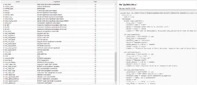
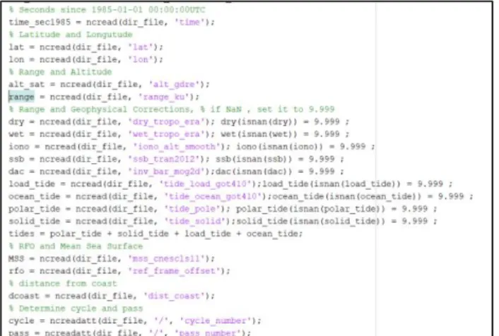
2.1 Pengecekkan Data RADS

Tahap awal yang dilakukan dalam pengolahan data adalah pengecekkan parameter data satelit

Jason-2 dan Jason-3 yang berformat .nc. Dalam pengolahan SSH dibutuhkan data altitude, koreksi

dry trophosperic, wet troposperic, ionosphere, tides, sea state bias, Dynamic Atmospheric

Correction dan RFO. Untuk pengolahan data SLA diperlukan SSH, dan MSS (Mean Sea Surface).

Dalam RADS banyak model koreksi yang disediakan, model koreksi yang digunakan untuk

penelitian ini adalah seperti pada Gambar 2.1. Selain itu juga diperlukan waktu pengambilan data.

Data waktu diambil dalam format MJD (Modified Julian Date) dan fraction of year.

Gambar 2.1. Pengecekan Data RADS

2.2 Perhitungan SSH dan SLA

Perhitungan SSH dan SLA dilakukan setelah melakukan pembacaan data .nc dan pengambilan variabel-variabel yang digunakan untuk menghitung SSH dan SLA. Berikut adalah script pembacaan data .nc.

Gambar 2.2. Script Pembacaan Data .nc

Perhitungan nilai SSH dilakukan menggunakan perangkat lunak MATLAB. Nilai SSH merupakan tinggi permukaan laut yang tereferensi pada ellipsoid. SSH) dengan script sebagai berikut.

Gambar 2.3. Script Perhitungan SSH

Setelah didapatkan nilai SSH, dilakukan perhitungan nilai SLA. SLA menggambarkan perbedaan antara ketinggian permukaan laut (SSH) dengan ketinggian muka laut rata-rata (MSS) dimana efek dinamis dan pengaruh atmosfernya sudah dihilangkan. Kemudian, SLA dihitung setiap pass dalam 1 cycle. SLA yang diambil dibatasi dengan kriteria yang tertera pada tabel berikut.

Tabel 2.1. Kriteria Kontrol Kualitas Data (Scharroo 2018)

Parameter Kriteria

Sea Level Anomaly -2,00 m < x(m) < 2,00 m

Dry Tropospheric -2,40 m < x(m) < 2,10 m

Wet Tropospheric -0,60 m < x(m) < 0,05 m

Ionosphere -0,40 m < x(m) < 0,04 m

Sea State Bias -1,00 m < x(m) < 1,00 m

Atmospheric Correction -1,00 m < x(m) < 1,00 m Ocean Tide -5,00 m < x(m) < 5,00 m Load Tide -0,50 m < x(m) < 0,50 m Solid Tide -1,00 m < x(m) < 1,00 m Pole Tide -0,10 m < x(m) < 0,10 m

Nilai koreksi yang bernilai 9,999 m yang tertera pada Gambar (2.1) dianggap NaN (Not a Number) untuk menghilangkan nilai yang kosong dan nilai lonjakan signifikan baik tinggi maupun rendah. Hasil SLA dan koreksi yang outlayer tidak akan digunakan. Berikut adalah script perhitungan SLA.

Gambar 2.4. Script Perhitungan SLA

Adapun hasil dari perhitungan SSH dan SLA didapatkan dengan file output dengan format text file (.txt) sebagai berikut.

Gambar 2.5. Hasil Perhitungan SSH dan SLA

Berdasarkan Gambar (2.5) dihasilkan nilai cycle, pass, MJD, latitude, longitude, SSH, SLA, MSS,

dry, wet, iono, SSB, tides, DAC, distance coast, dan YYF (fraction of year). Satuan SSH dan SLA yang

digunakan pada tahap ini adalah meter.

2.3 Rata-rata SLA per cycle

Jumlah cycle yang digunakan untuk Jason-2 sebanyak 303 cycle dan Jason-3 sebanyak 106

cycle. Tiap cycle terdiri dari beberapa pass yang mempunyai nilai berbeda setiap pass seperti pada

Gambar (4.6). Maka dari itu dilakukan perhitungan rata-rata nilai MJD, SSH, SLA dan YYF untuk

mengetahui besar nilai tersebut untuk setiap cycle nya.

Perhitungan rata-rata yang dilakukan dibobotkan menurut lintangnya. Pembobotan menurut

Berikut adalah script perhitungan rata-rata SLA per cycle.

Gambar 2.6. Script Perhitungan Rata-rata SLA

Nilai rata-rata semua SLA adalah 116,144 mm. Untuk SLA tertinggi pada cycle 86 Jason 2 sebesar

211,723 mm. Nilai SLA terendah pada cycle 268 Jason 2 sebesar 19,509 mm.

2.4 Intercalibrated Tandem Mission

Interkalibrasi dilakukan karena adanya tandem mission satelit Jason-2 dan Jason-3. Tandem

mission adalah pengambilan data oleh 2 satelit dalam periode waktu yang sama dengan jalur yang

sama, sehingga terjadi penumpukan akuisisi data.

Data rata-rata per cycle dibuat untuk mengetahui dimana letak tandem mission ini. Dapat

dilihat pada Gambar 2.7.

Gambar 2.7. Grafik Time Series SLA sebelum Interkalibrasi

Dari grafik diatas diketahui bahwa tandem mission untuk Jason-2 dan Jason-3

masing-masing terjadi pada cycle 281-303 (J2) dan cycle 1-23 (J3). Berikut adalah visualisasi dalam bentuk

grafik sebelum dan sesudah dilakukan interkalibrasi pada Jason-2 dan Jason-3.

Gambar 2.8. Grafik SLA Terinterkalibrasi

Setelah diketahui rentang cycle yang mengalami tandem mission, dilakukan perhitungan bias. Bias dihitung dengan hitung perataan yaitu selisih SLA antara Jason-3 dan Jason-2 per cycle dihitung kemudian dirata-rata. Nilai bias mean SLA antara Jason-2 dan Jason-3 adalah 3.757 mm, sedangkan untuk bias mean SSH sebesar 169.640 mm. Setelah didapatkan nilai bias kemudian nilai SLA Jason-3 dikoreksikan. Hasil SLA terkoreksi dapat dilihat pada Gambar 2.9.

Dari proses diatas data yang digunakan pada proses selanjutnya adalah cycle 1 hingga 290 (J2) dan

Gambar 2.9. Grafik Time Series SLA Sesudah Interkalibrasi

2.5

Gridding

Gridding dilakukan pada data SSH, SLA, dan arus model. Tahap ini dilakukan menggunakan software Surfer. Gridding SLA dan SSH dilakukan dengan metode data metric (z=mean) dan ukuran grid yang digunakan adalah 3°x3°. Ukuran ini disesuaikan dengan jarak antar lintasan satelit altimetri yaitu sebesar 315 km (±3°). Grid dihitung untuk setiap cycle dengan format akhir data (.gdr). Batas wilayah yang digunakan 20LU -20 LS dan 90 BT -150 BT maka hasil titik grid yang dihasilkan adalah melintang 14 baris dan membujur 21 baris.

Gambar 2.10. Hasil Gridding pada Surfer

Data gridding diubah formatnya dari .grd menjadi .txt agar dapat muncul angka pada setiap grid sehingga dapat dilanjutkan untuk perhitungan korelasi nantinya. Berikut adalah hasil export data (.gdr) menjadi (.txt).

Data arus model di gridding menggunakan software Ocean Data View dengan ukuran grid yang sama SLA. Metode yang dirasa menghasilkan data mendekati arus hitungan dengan ukuran grid yang sama.

2.6 Perhitungan Arus

Perhitungan arus dapat dimulai ketika telah didapatkan nilai SSH terkoreksi, ter-interkalibrasi dan telah ter-gridding . Data dikelompokkan setiap bulan dalam satu tahun mulai bulan Januari hingga Desember pada rentang tahun 2009-2018. Elemen yang dihitung untuk mendapatkan kecepatan dan arah arus geostropik adalah u dan v. Masing-masing komponen tersebut dihitung. Perhitungan dilakukan dengan perangkat lunak Matlab dan Ms. Excel.

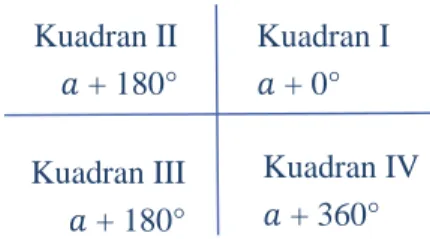
Setelah didapatkan u dan v, proses selanjutnya adalah menghitung kecepatan arus Arah arus laut dihitung dengan menggunakan kuadran aritmatik seperti pada Gambar 2.11 berikut.

Gambar 2.11. Kuadran Aritmatik

Dimana a adalah sudut yang dihasilkan. Perhitungan arus dilakukan perbulan dalam setiap tahun selama kurun waktu 2009-2018.

Kuadran I 𝑎 + 0° Kuadran II 𝑎 + 180° Kuadran III 𝑎 + 180° Kuadran IV 𝑎 + 360°

BAB III STATUS LUARAN

Dalam penelitian laboratorium dana local ITS, target luaran utama adalah publikasi pada jurnal

internasional terindeks, dalam hal ini jurnal internasioanal terindeks Q2. Proses penulisan jurnal

sedang dilakukan.

Selain itu, hasil dari penelitina ini telah di presentasikan dalam Seminar Internasional GEOICON

2020 yang telah dilakukan pada tanggal 26 Agustus 2020, dengan penyelengaranya adalah

Departemen teknik Geomatika ITS. Seminar internasional ini akan di publikasikan pada proseding

internasional terindeks.

BAB IV KENDALA PELAKSANAAN PENELITIAN

Dalam pelaksanaan penelitian ini secara umum berjalan dengan baik, walaupun harus dikerjakan di

rumah karena adanya pandemic covid 19.

BAB V RENCANA TAHAPAN SELANJUTNYA

Sesuai target luaran penelitian ini adalah publikasi pada jurnal internasional terindeks Q2, Tim peneliti sedang mempersiapkan penulisan publikasi. Rencana publikasi akan dilakukan pada Jurnal “Terrestrial,

BAB VI DAFTAR PUSTAKA

[1] Marpaung, S., Prayogo, T. 2014. Analisis Arus Geostropik Permukaan Laut Berdasarkan

Data Satelit Altimetri. Seminar Nasional Penginderaan Jauh.

[2] Gordon, A.L. and R.A. Fine. 1996. Pathways of water between the Pacific and Indian

Oceans in the Indonesian Seas. Nature, 379 (6561):145-149.

[3] Gordon, A.L. 2005. Oceanography of the Indonesian Seas and Their Through Flow.

Oceanography, 18(4):14-27.

[4] DUXBURY, A; B. ALYN; C. DUXBURY and K.A. SVERDRUP 2002. Fundamentals of

Oceanography-4th Ed, McGraw-Hill Publishing, New York.

[5] Evelyn Brown et al, Angela Colling(editor). 2001. Ocean Circulation 2

nd

_{Edition. Open}

University

[6] Hadi, S. and I.M. Radjawane. 2009. Sea Currents. College Book. ITB: Department of

Oceanography.

[7] M. Furqon Azis. 2006. GERAK AIR DILAUT. Oseana. 31(4): 9 – 21

[8] Handoko, E. Y. 2004. Satelit Altimetri dan Aplikasinya Dalam Bidang Kelautan. Scientific

Journal, Pertemuan Ilmiah Tahunan I. Teknik Geodesi – ITS, Surabaya, Indonesia , 2004.

[9] Oktavia, R, J.I. Pariwono and P. Manurung. 2011. Variation of Sea Surface and Surface

Geostrophic Current in Sunda Strait waters based on Tidal Wave and Wind Data year

2008. Journal of Topical Marine Science and Technology Vol.3 (2):127

[10] Ramadyan, Fachri and Ivonne M.Radjawane. 2013. Seasonal Surface Geostrophic Current in

the Arafura – Timor Sea. Journal of Tropical Marine Science and Technology Vol.5

(2):261-271.

[11] Harini, W.S. 2004. Pola Arus Permukaan di Wilayah Perairan Indonesia dan Sekitarnya

yang diturunkan Berdasarkan Data Satelit Altimetri TOPEX/POSEIDON. Tesis. IPB.

[12] Marthin Matulessy. 2014. Dinamika Tinggi Paras Laut dan Pola Arus Geostropik dari

Data Satelit Altimetri di Perairan Selatan Jawa. Thesis. Tidak Diterbitkan. Program Studi

Kelautan, Institut Pertanian Bogor.

[13] Stewart, R. H. 2008. Introduction to Physical Oceanography, pdf version. Departement of

Oceanography. Texas A & M University.

[14] Rahman, Abdul A.,2007. Identifikasi hubungan fluktuasi nilai soi terhadap curah hujan

bulanan di kawasan Batukaru-Bedugul, Bali.Jurnal bumi lestari . Vol. 7(2):123129

BAB VII LAMPIRAN

Lampiran berisi tabel daftar luaran (Format sesuai lampiran 1) dan bukti pendukung luaran wajib dan luaran tambahan (jika ada) sesuai dengan target capaian yang dijanjikan

LAMPIRAN 1 Tabel Daftar Luaran

Program

: Penelitian Pascasarjana

Nama Ketua Tim

: Dr. Eko Yuli Handoko, ST., MT

Judul

: Studi Pola Arus Geostopik di Perairan Indonesia

menggunakan Data Satelit Altimetri Jason-2 dan Jason-3

1.Artikel Jurnal

No

Judul Artikel

Nama Jurnal

Status Kemajuan*)

1

Variability of Sea Level Around

the Indonesian Seas and its

Correlation with ENSO and

Indian Ocean Dipole

Terrestrial,

Atmospheric and

Oceanic Sciences

Persiapan

*) Status kemajuan: Persiapan, submitted, under review, accepted, published

2. Artikel Konferensi

No

Judul Artikel

Nama Konferensi (Nama

Penyelenggara, Tempat,

Tanggal)

Status Kemajuan*)

1

Altimetry-derived Geostrophic

Current around the Indonesian

Seas

GEOICON2020,

DEpartemen Teknik

Geomatika ITS,

Surabaya, 26 Agustus

2020

Presented

*) Status kemajuan: Persiapan, submitted, under review, accepted, presented

3. Paten

No Judul Usulan Paten

Status Kemajuan

-

*) Status kemajuan: Persiapan, submitted, under review

4. Buku

No

Judul Buku

(Rencana) Penerbit

Status Kemajuan*)

-

*) Status kemajuan: Persiapan, under review, published

5. Hasil Lain

No

Nama Output

Detail Output

Status Kemajuan*)

-

6. Disertasi/Tesis/Tugas Akhir/PKM yang dihasilkan

No Nama Mahasiswa

NRP

Judul

Status*)

1

Desi Suci Richasari

03311640000008

Analisis Arus Geostropik

di Perairan Indonesia

Menggunakan Data

Satellit Altimetri Jaon-2

dan Jason-3

Lulus – 2020

2

Fajar Kharisma

03311750012002 Studi Variasi Seasonal

dan Annual Permukaan

Laut di Indonesia

Menggunakan data Satelit

Altimetri

In progress

Altimetry-derived Geostrophic Current around the

Indonesian Seas

Eko Yuli Handoko, Desi Suci Richasari, Danar Guruh Pratomo, M. Nur Cahyadi

Department of Geomatics Engineering, Institut Teknologi Sepuluh Nopember, Surabaya, Indonesia 60111

Corresponding email: ekoyh@geodesy.its.ac.id

Abstract. This research aimed to determine and analyze the geostrophic current towards the

monsoon index and the El Nino South Oscillation index. The location of this research is around Indonesian seas with coordinates of 20 ° N - 20 ° S latitudes and 90 ° E - 150 ° E longitudes. Jason Series altimetry satellite data are beneficial as a provider of data on global marine affairs, including information about sea surface and sea level currents. To determine the geostrophic current, we used the geostrophic algorithm. The analysis method used the coefficient correlation of the results between the research parameters and the index—temporal and spatial analysis using MATLAB, and ArcMap visualizes the parameters obtained. This study indicates that the correlation between sea level anomaly and the Multivariate ENSO Index shows a negative value. It means that Sea Level Anomaly at Indonesian seas had an opposite condition when El Nino happened, Sea Level Anomaly is lower than when La Nina happened, and Sea Level Anomaly is high. The strong El Nino occurred in 2015, and La Nina occurred in 2010. The SLA difference does not affect the direction of the geostrophic current but affects its velocity. The correlation of zonal component geostrophic current to the Australian Monsoon Index is 0,720, and Western North Pacific Monsson Index is 0,446. It means that the geostrophic current has the same direction as the wind flow, respectively, during the monsoon season.

1. Introduction

Circulation and seawater dynamics occur continuously, and it exists at the surface and in the deep. One of the circulations is sea currents [1]. The general surface currents in the Indonesian Seas are affected by the northwest and southeast monsoon cycle, which changes periodically. It causes seasonal changes in oceanographic parameters such as density, temperature, and salinity [2].

According to reference [3], the Indonesian sea has an area ± 5,9 km². It is flanked by the Pacific Ocean and the Indian Ocean. The difference in air mass between the two oceans causes a mass flow of water from the Pacific Ocean to the Indian Ocean, known as Indonesian Through Flow (ITF). The ITF has a significant impact on sea surface temperature, the freshwater budget, and the climate system [4]. Currents (water mass flow) play an essential role in the global climate [5]. The type of ocean currents that affect global is geostrophic current.

Geostrophic current is current that occurs due to geostrophic balance. Reference [6] states that the geostrophic balance occurs when the Coriolis force balances the horizontal pressure gradient due to earth movement. These currents are related to higher sea level slope with lower built by Ekman transport [7]. Ekman transport is a mass transport of water whose direction is perpendicular with wind direction

to the right in the northern hemisphere and to the left in the southern hemisphere is related to the rate of change of current with depth [8]. Therefore, current movements are related to sea level.

Sea level or Sea Surface Height (SSH) is sea level height differentiated in the reference ellipsoid. With the development of altimetry, satellite technology is an alternative to fulfill oceanographic data such as sea level and other ocean dynamics, both regional and global. SSH data can derive surface geostrophic flow patterns.

There have been many studies on the variability of geostrophic currents, not yet done for the Indonesian sea. Research on sea surface variations and surface geostrophic have been carried out in the Arafura Sea and Sunda Strait, where variations in the Sunda Strait surface are found that cause rainy seasons [9]. Research on variations in the flow of geostrophic currents in Arafura-East waters found the dynamics of geostrophic currents in Arafura-East waters occurring sea-level changes due to the monsoon every season [10]. The results of this study stated that it greatly affects the variability of geostrophic currents. Another factor that plays a role in the circulation of geostrophic currents is ITF [4].

Because Indonesia's location is strategic, transitions by monsoons that encounter periodically throughout the year, it is necessary to research sea-level dynamics and geostrophic currents to advance the dynamics distribution of sea level height anomalies and spatial and temporal flow patterns. Analysis of sea-level changes is done by considering zonal (u) and meridional (v) components represented in monthly periods—then correlated with MEI and Moonson Index.

2. Data and Methods

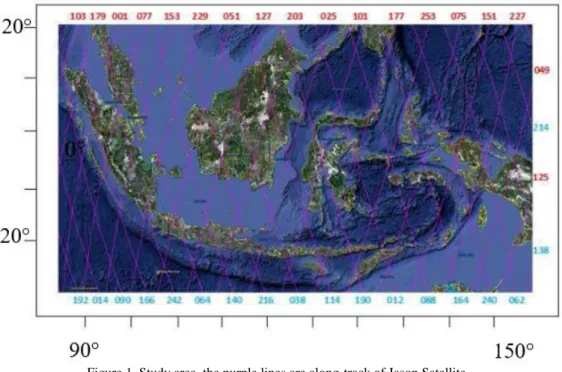
2.1. Study Area

The location of this research was restricted in Indonesian seas with coordinates of 20 ° North - 20 ° South latitudes and 90 ° -150 ° East Longitude. The research location can be seen in Figure 1.

Figure 1. Study area, the purple lines are along-track of Jason Satellite

2.2 Data and Methods

Geostrophic currents and sea surface height used is derived by altimetry data Jason-2 and Jason-3. The data have been corrected for all geophysical corrections: ionospheric, dry, and wet tropospheric delays, sea state bias, solid Earth, ocean and pole tides, ocean tide loading, and inverted barometer correction. According to [11], a simple formulation to calculate the Sea Surface Height (SSH) as following:

𝑆𝑆𝐻 = 𝐻 − 𝑅 ̂ (1) Where H is satellite height above ellipsoid (altitude), 𝑅 ̂ is the corrected range.

Several indices monitor the tropical Pacific phenomenon, all of which are based on sea level anomaly (SLA) average across a given region. The Multivariate ENSO Index (MEI) is the most commonly used indices to define El Nino and La Nina events where the MEI v.2 typically uses bi-monthly running mean, and El Nino or La Nina events are defined as when the MEI v.2 SLA exceeds +/-0.5. When it is greater than 0.5, it is expressed as the El Niño period, when lower than -0.5, and then is expressed as La Niña period, respectively. In this study, we used the bi-monthly data of MEI v.2 from NOAA to determine the Elnino and La Nina episodes, where the SLA was taken toward the bi-monthly of MEI v.2 during the period 2008-2018.

The data of geostrophic current at the sea surface consist of two components such as u and v. The geostrophic current velocity obtained from the calculation using the formula below [12]:

𝑢 = −𝑔_𝑓𝜕𝑦𝜕𝜁 𝑣 =𝑔_𝑓𝜕𝑥𝜕𝜁 (2) Where u is the zonal surface geostrophic current velocity (m/s), v is the meridional surface geostrophic current velocity (m/s), 𝜁 absolute dynamic topography (m), g is gravity (m/s²), and f is the Coriolis parameters. Then the result was validated by the geostrophic current component from Copernicus Marine Service (CMEMS). Then, we calculate the geostrophic current velocity results to compare with the wind velocity provided by ECMWF.

We also calculate the correlation between the zonal surface geostrophic current to the monsoon index's value, especially the Australian Monsoon Index (AUSMI) and Western North Pacific Monsoon (WNPMI) Index. Also, correlation analysis was performed on the SSH and SLA difference between the western Pacific Ocean and the eastern Indian Ocean to the occurrence of ENSO. The correlation equation is the Pearson correlation, which s formulated as follows:

(3)

Where 𝜚𝑥𝑦is the Pearson correlation, 𝜎𝑥𝑦 is the covariance of XY., 𝜎𝑥 is the standard deviation of x,

𝜎𝑦 is the standard deviation of y, 𝜇𝑥is mean of x, 𝜇𝑦 is mean of y, n is the amount of sample, X is the

independent variable, Y is the dependent variable. The relationship between the variables in the correlation analysis is based on the values in Table 1 below.

Table 1. Interpretation of Correlation Coefficient [13]

Interval Level of relationship

0,80≤ 𝜚𝑥𝑦≤1,00 Very Strong

0,60≤ 𝜚𝑥𝑦<0,80 Strong

0,40≤ 𝜚𝑥𝑦<0,60 Moderate

0,20≤ 𝜚𝑥𝑦<0,40 Low

3. Results and Discussion

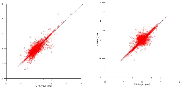
3.1. Validation of Geostrophic Current Data

Validation is performed by calculating the current data and the current model that has been downloaded previously. In Figure 2, it is a graph between the data model and the calculated data where there are stretched data in the middle of 2015-2016; the rest of the patterns of the two graphs show similarity. The estimated value is for component u, respectively 0.715, and for component, v is 0.331. With RMSE component u is 0,217 and component v is 0,180. Small RMS-error indicates that the data model and data count have low data value differences. It means we can go to the next step.

Figure 2. Scatter Plot of U, V Calculated and U, V Model

3.2. Modeling of Geostrophic Current Pattern

Geostrophic current modeling is done with the observation period 2009-2018, which has been grouped monthly based on seasonal patterns. Seasonal patterns in the tropics are divided into two, namely Northwest Season (December, January, February) and Southeast Season (June, July, August). Transition Season I (March, April, May) and Transition Season II (September, October, November).

3.2.1 West Monsoon

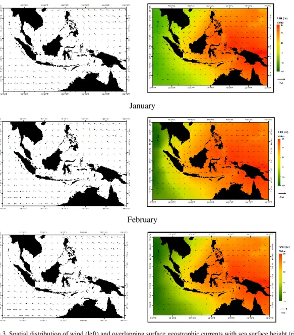
Figure 3 displays wind patterns and current patterns spatially in Indonesian waters during the west monsoon period. Generally, in this period, winds from the northwest to the east for 5 ° north-5 ° south latitudes, the average speed is 4.50 m / s with the dominant wind speed in January. The pattern is almost the same as shown by the current, wherein the Pacific Ocean the wind originates from east to west, entering Indonesian waters through the Makassar Strait and the Maluku Sea then southward and turning west towards the Indian Ocean. This current is known as Indonesian Through Flow (ITF). The average current velocity in the west season is 0.217 m / s, and the most significant average velocity in January. It makes January's winds and currents peak at the West Season with the strongest magnitude.

Ocean currents flow from the high SSH to the common SSH [14]. High SSH is marked in orange and common SSH is marked in green with values ranging from 85m to -65m. Based on Figure 3, The

Andaman Sea and the Indian Ocean have relatively low SSH. However, currents at 0 ° - 5 ° latitude point to a higher SSH, from the Andaman Sea and the Indian Ocean to the Sunda Strait and the Java Sea. Flow from the South China Sea with a higher SSH towards Indonesia via the Karimata Strait towards the north of the Java Sea with a lower SSH. Likewise, the Pacific Ocean with high SSH flowing through the Makassar Strait and the Maluku Sea towards the Indian Ocean with a low SSH.

December

January

February

Figure 3. Spatial distribution of wind (left) and overlapping surface geostrophic currents with sea surface height (right) at Indonesian Seas in the Northwest Season (label not so clear)

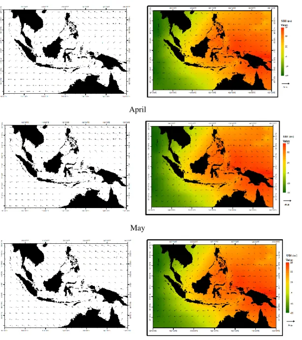
3.2.2 Transition Season 1

The current and wind patterns during Transition Season I are shown in Figure 4, the transition from the Northwest Season to the Southeast Season caused a weakening in both the current and wind. This period's average wind speed was 3.952 m / s and 0.17 m / s for the current velocity. Flow in March and April at latitude 5 ° north - 10 ° south latitudes the dominant current heading east. In contrast to the dominant direction of the wind to the west. In May, changes in the direction of wind and currents occur. Winds from the southeast, at the equator, is turn left. The southeast to the east coast was split into two

parts, to the Indonesian seas and the Indian Ocean. The current flows into Indonesian seas through the Flores Sea, the Java Sea, and north towards the Karimata Strait.

March

April

May

Figure 4.Spatial distribution of wind (left) and overlapping surface geostrophic currents with sea surface height (right) at Indonesian Seas during the Transition Season I

3.2.3 East Season

Wind patterns and currents of the East Season are shown in Figure 5. This picture shows wind patterns from the east and southeast and currents that generally head west and northwest. This season's

wind has a high value in its annual cycle. Average wind speed of 4,913 m / s. Currents have a dominant magnitude: north of Papua, the Banda Sea, the Seram Sea, and the Maluku Sea. This current is known as the Papua Coastal Current (NGCC), a current that runs along the northern coast of Papua and originates from the southern Pacific Ocean.

June

July

August

Figure 5. Spatial distribution of wind (left) and overlapping surface currents with sea surface height(right) at Indonesian Seas during the East Season

3.2.4 Transition Season II

Figure 6 shows the current and wind patterns in the transition season II, and this season is a transition from the East Season to the West Season, represented by September, October, and November. The

direction of the current that occurs in this season is still dominant towards the west and northwest as in the east season, which occurs at latitude 10 ° north -20 ° north latitude and 10 ° south - 20 ° south latitude. Slowly the current velocity is weakening from September to October and starts to rise in November.

September

October

November

Figure 6. Spatial distribution of wind (left) and overlapping surface geostrophic currents with sea surface height (right) at Indonesian Seas during the Transition Season II

3.3. Correlation with The Index

3.3.1 Correlation between SLA and MEI

The correlation between SLA and MEI is -0.66 (negative correlation), so the relationship between the two variables is strong but inversely proportional. El Nino occurs when the MEI value is positive, and La Nina occurs when the MEI value is negative. Based on Figure 7, a strong El Nino event occurred in 2015, and a strong la Nina occurred in 2010-2011. There was an increase in SLAs in general, but there was a decrease when El Niño happened. When La Nina (2010) occurred, the condition of SLA in the Pacific Ocean was lower than in the Indian Ocean region, according to reference [15].

Figure 7. The relation between SLA and Multivariate ENSO Index v.2

3.3.2 Geostrophic current Velocity and MEI

The correlation between the average geostrophic current velocity and MEI is 0.24. This result shows that the relationship between the two variables is weak and goes in the same direction. The average speed of geostrophic currents in Indonesian waters at El Nino is higher than at La Nina. The difference in current velocity when El Nino (2015) and La Nina (2010) occurs is 0.54 m / s. The highest current speed conditions when El Nino SLA in the Pacific Ocean is lower than in the Indian Ocean.

Figure 8. Geostrophic current velocity during the ENSO in 2009 -2018 (yellow should be written at figure caption)

3.3.3 Zonal current and AUSMI

The AUSMI index is an index of monsoon eastern wind (Australia), which carries dry clouds. Determination of the east wind index's influence can be seen from the direction of the zonal current,

Warm Cold SLA Warm Cold Geostrophic Velocity

namely the sign (-) of the west monsoon wind and (+) the east monsoon wind. So, the month marked (+) is influenced by the east monsoon wind. Table 2 is the result of a comparison of zonal flows from 2009 to 2015 and the AUSMI index value.

Table 2. Zonal Current and AUSMI Index 2009-2015

Year Month Zonal

Current (u) (m/s) AUSMI Index 2009 December -0.027 -0.161 2009 January -0.006 0.434 2009 February -0.035 0.427 2010 December -0.003 1.092 2010 January -0.007 0.579 2010 February -0.053 -0.645 2011 December -0.012 0.122 2011 January -0.002 1.491 2011 February 0.001 0.911 2012 December -0.061 -1.200 2012 January -0.002 0.127 2012 February -0.046 -1.563 2013 December -0.037 -0.492 2013 January -0.015 0.758 2013 February -0.042 -0.424 2014 December -0.008 -0.244 2014 January -0.007 0.769 2014 February -0.001 0.388 2015 December -0.005 0.895 2015 January -0.046 1.041 2015 February -0.049 -1.277

The results of current zonal processing to the AUSMI index produce a correlation coefficient of 0.720, classified in a very strong classification. The zonal current velocity in the rainy season ranges from 0.061 to 0.001 m / s with a maximum speed occurring in December 2012 of 0.061 m / s and a minimum speed occurring in February 2011 and 2014 of 0.001 m / s. February 2011 with a velocity (+) of 0.001 and an index value of 0.911 indicates that the influence of the east monsoon wind in that month, a significant enough index value indicates lower rainfall.

3.3.4 Zonal Current and WNPMI

The WNPMI index influences the variability of rainfall only during the rainy season. A negative sign (-) indicates a moving wind from west-east (western(-) or west monsoon (Asia(-), and a positive sign (+(-) indicates a moving wind from east-west (eastern) or east monsoon (Australia). Table 3 shows the comparison of zonal flows from 2009 to 2015 and WNPMI index values.

Table 3. Zonal Current and WNPMI Index

Year Month Zonal

Current (u) (m/s) WNPMI Index 2009 June -0.032 0.579 2009 July -0.038 1.018 2009 August -0.034 0.068

2009 September -0.012 2.075 2010 June -0.090 -1.117 2010 July -0.082 -1.805 2010 August -0.053 -0.395 2010 September -0.076 -2.113 2011 June -0.041 0.480 2011 July -0.046 0.657 2011 August -0.077 -0.188 2011 September -0.059 1.037 2012 June -0.020 1.410 2012 July -0.066 0.796 2012 August -0.064 0.604 2012 September -0.052 0.467 2013 June -0.034 -0.029 2013 July -0.065 -0.201 2013 August -0.052 -0.156 2013 September -0.033 1.336 2014 June -0.026 0.194 2014 July -0.005 1.605 2014 August -0.049 -1.335 2014 September -0.017 -0.546 2015 June -0.036 -0.892 2015 July -0.061 0.386 2015 August -0.007 -0.642 2015 September -0.023 -0.910

The results of current zonal processing to the WNPMI index produce a correlation coefficient of 0.446, which is classified as a weak classification. It means that the WNPMI index has little effect on zonal currents. The zonal current velocity in the dry season ranges from 0.090 to 0.005 m / s, with a maximum speed occurring in June 2010 of 0.090 m/s and the minimum speed occurring in July 2014 of 0.0005 m/s. Zonal current velocity from June to September 2009-2015 shows a negative value (-), which means that in those months, it is still influenced by the West Munson wind, which carries much water with a small intensity. The lowest rainfall was in July 2010, with the smallest WNPMI index value of -1.805. It was considering that in 2010 La Nina was the strongest. The highest WNPMI index was in July 2014, with a zonal flow velocity of 0.005 m/s.

3.4. Temporal analysis between Sea Level Anomaly and Geostrophic Current

The results of the annual SLA periodogram show that some patterns are consistent. The strong annual pattern in November-January and annual pattern in July-October. It shows that annual and semi-annual climate characteristics dominate Indonesian waters. Based on Figure 9, Indonesian Seas have a dominant rainy season with maximum frequency (intensity) in November-January, decreasing in December and increasing again in January. In contrast, the dry season is indicated when the low frequency occurs in March-June.

4. Conclusion

In this study, the geostrophic current around the Indonesian sea has been performed using Jason2 and Jason-3 satellite altimetry data. The correlation value between the geostrophic current from CMEMS and satellite altimetry for the component u is 0.715, and component v is 0.331. Geostrophic currents have a pattern in each season at The West Season, Transition Season I, East Season, and Transition Season II. The correlation coefficient of correlation between SLA and MEI of -0.66 (negative correlation), the level of relationship between the two variables is strong but inversely proportional. It means that the ENSO phenomenon affects sea level anomalies in Indonesian waters. Meanwhile, the correlation between the average geostrophic current velocity and MEI is 0.24, meaning that the ENSO phenomenon has a weak influence on the geostrophic current velocity. Meanwhile, the processing of zonal currents to the AUSMI index produces a correlation coefficient of 0.720, classified as a robust correlation.

Acknowledgment

This research was funded by the Directorate of Research and Community Service, Institut Teknologi Sepuluh Nopember, Ministery Education and Culture, following the ITS Fund Postgraduate Research implementation Agreement 2020 number 919/PKS/ITS/2020, date of 02nd _{April 2020}

References

[1] Marpaung, S., Prayogo, T. 2014. Analisis Arus Geostropik Permukaan Laut Berdasarkan Data Satelit Altimetri. Seminar Nasional Penginderaan Jauh.

[2] Gordon, A.L., and R.A. Fine. 1996. Pathways of water between the Pacific and Indian Oceans in the Indonesian Seas. Nature, 379 (6561):145-149.H. Poor, An Introduction to Signal Detection and Estimation. New York: Springer-Verlag (1985) Ch. 4.

[3] Lasabuda, R. (2013). PEMBANGUNAN WILAYAH PESISIR DAN LAUTAN DALAM PERSPEKTIF NEGARA KEPULAUAN REPUBLIK INDONESIA. Jurnal Ilmiah Paltax, 92-101.

[4] Gordon, A.L., 2005. Oceanography of the Indonesian Seas and Their Through Flow. Oceanography, 18(4):14-27.J. Wang, "Fundamentals of erbium-doped fiber amplifiers arrays (Periodical style—Submitted for publication)," IEEE J. Quantum Electron., [5] DUXBURY, A; B. ALYN; C. DUXBURY and K.A. SVERDRUP 2002. Fundamentals of Oceanography-4th Ed, McGraw-Hill

Publishing, New York.

[6] Ablain, M., P. Escudier, A. Couhert, Flavien M., Alain Mallet, P. Thibaut, Ngan Tran, L. Amarouche, Bruno Picard, L. Carrere, G. Dibarboure, J. Richard, Nathalie Steounou, P. Dubois, M. H. Rio, dan J. Dorandeu. 2018. Satellite Radar Altimetry: Principle, Accuracy, and Precision. In Cazenave, A., dan Detlef Stammer (Eds.), Satellite Altimetry Dover Oceans and Land Surface. CRC Press: ISBN-13 [7] Hadi, S., and I.M. Radjawane. 2009. Sea Currents. College Book. ITB: Department of Oceanography.

[8] Jacob O. Wenegrat, L. N. (2017). Ekman Transport in Balanced Currents with Curvature. Journal of Physical Oceanography, 1189-1203.

[9] Oktavia, R, J.I. Pariwono, and P. Manurung. 2011. Variation of Sea Surface and Surface Geostrophic Current in Sunda Strait waters based on Tidal Wave and Wind Data year 2008. Journal of Tropical Marine Science and Technology Vol.3 (2):127S. P. Bingulac, "On the compatibility of adaptive controllers (Published Conference Proceedings style)," in Proc. 4th Annu. Allerton Conf. Circuits and

Systems Theory, New York (1994) 8–16.

[10] Ramadyan, Fachri, and Ivonne M.Radjawane. 2013. Seasonal Surface Geostrophic Current in the Arafura – Timor Sea. Journal of Tropical Marine Science and Technology Vol.5 (2):261-271.

[11] Andersen, O.B., dan Scharroo, R. 2011. Range and Geophysical Corrections in Coastal Regions: and Implications for Mean Sea Surface Determination. In Benveniste, J., S. Vignudelli, Andrey G. Kostianoy, Paolo Cipollini (Eds.), Coastal Altimetry (Chapter 5: pp. 103– 145). Springer: Berlin/Heidelberg, Germany.

[12] H.A Rejeki, Kunarso dan Munasik, 2016. Interannual variability of sea surface height difference between the western Pacific Ocean and the eastern Indian Ocean and its effect to geostrophic current in Lombok Strait. IOP Conf. Series: Earth and Environmental Science 162 (2018)

[13] Evans, J D., 1996. Straightforward Statistic for the Behavioral Science. Pacific Grove, CA:Brook/Core Publishing.

[14] Chung, R. H., Zheng, Q., Soong, Y. S., Nan, J. K., and Jian, H. H., 2000, Seasonal variability of sea surface height in the South China Sea observed with TOPEX/Poseidon altimeter data. Journal of Geophysical Research, 105, pp 13,981-13,990.

[15] Hndoko, E., Y. , Hariyadi. H. (2018). The ENSO's Influence on the Indonesian Sea Level Observed Using Satellite Altimetry, 1993 - 2016. IEEE Asia-Pacific Conference on Geoscience, Electronics, and Remote Sensing Technology (AGERS).