LAPORAN PENELITIAN
MACRO INDICATORS IMPACT TOWARDS RESIDENTIAL ELECTRICITY CONSUMPTION IN INDONESIA
Oleh:
Yusak Tanoto, S.T., M.Eng. Maria Praptiningsih, S.E., M.Sc.F.E
ELECTRICAL ENGINEERING DEPARTMENT- BUSSINESS MANAGEMENT PROGRAM
PETRA CHRISTIAN UNIVERSITY SURABAYA
Halaman Pengesahan
1 Judul Penelitian : Macro Indicators Impact Towards Residential
Electricity Consumption in Indonesia 2 Ketua Peneliti:
a. Nama Lengkap dan Gelar : Yusak Tanoto, S.T., M.Eng.
b. Jenis Kelamin : L
c. NIP : 04-020
d. Jabatan Fungsional : Lektor
e. Jurusan/Fakultas/Pusat Studi : Teknik Elektro/Fakultas Teknologi Industri
f. Telepon kantor & HP : 2983445 & 083853941599
g. E-mail : [email protected]
h. Alamat Rumah : Citra Melati 80 Tropodo, Sidoarjo
3 Jumlah Anggota Peneliti : 1
a. Nama Anggota Peneliti I : Maria Praptiningsih, S.E., M.Sc.F.E.
Fakultas/Jurusan : Fakultas Ekonomi/Manajemen Bisnis
b. Nama Anggota Peneliti II : -
Fakultas/Jurusan : -
4 Lokasi Penelitian : Universitas Kristen Petra
5 Institusi lain yang bekerjasama : -
6 Jangka Waktu Penelitian : 8 bulan
7 Biaya yang diusulkan
a. Sumber dari UK Petra : Rp. 10.720.000,-
b. Sumber lainnya : -
Total : Rp. 10.720.000,-
Surabaya, 2 Juli 2012
Mengetahui,
Dekan Fakultas Teknologi Industri Ketua Peneliti
Ir. Djoni Haryadi Setiabudi, M.Eng. Yusak Tanoto, S.T., M.Eng.
NIP: 85-009 NIP: 04-020
Menyetujui: Kepala LPPM UK Petra
Abstract
Household electricity consumption has become the highest rank among other sectors in Indonesia over the past decade. Its consumption growth takes second place after industrial sector with 8.14% and 10.45%, respectively, during 2006-2010. In the other hand, the importance of achieving the predetermined electrification ratio, as it reflects part of millennium development goal, has been unavoidable.
Macro indicators impact towards electricity consumption in the residential sector is then considered prominent to be investigated in relation to the energy policy planning. The research objective includes establishment of appropriate model containing macro indicators as the variables through the utilization of econometric method. The study period is 1990 – 2010. In addition, the forecasting model for household electricity consumption is also developed using econometric method. Factors decomposition is then used to obtain several types of effect contributed in the electricity consumption growth during 2000 – 2010, such as intensity effect, structural effect, as well as activity effect.
From the econometric point of view, the results found that BI rate, GDP, inflation and population are not significantly affecting the total energy consumption in Indonesia. Meanhile, electrification ratio and private consumption are significantly affecting to total energy consumption in Indonesia. In conclusion, total energy consumption has strongly influenced by the electrification ratio and private consumption. Moreover, the forecasting results found that the best model through ARIMA model in forecasting BI rate is ARIMA (0,1,1) or IMA (1,1); electrification ratio is ARIMA (1,1,0) or ARI (1); inflation is ARIMA (0,1,1) or IMA (1,1) and total energy consumption is ARIMA (0,1,1) or IMA (1,1). Similarly, the best model through ARCH/GARCH model in forecasting electrification ratio is ARCH (1) and GARCH (1); GDP is ARCH (1) and GARCH (1); Inflation is ARCH (1) and GARCH (1); and total energy consumption is ARCH (1) and GARCH (1).
Meanwhile, using Log Mean Divisia Index (LMDI) method which is offer more benefits over Aritmetic Mean Divisia Index (AMDI). Using LMDI additive-technique for the case of total residential sector of Indonesia, we find total residential electricity consumption in the period 1990 – 2010 became 29.285,2 GWh. The activity effect which is based GDP changes is the dominant factors contributing electricity consumption growth with 56.634,3 GWh. Insignificant contribution to the increasing electricity consumption was given by the structural effect changes in portion of household expenditure to the GDP, with 3.217.9 GWh in aggregate. On the other hand, intensity changes has consistently shown yearly negative value throughout the study period except for 2005 – 2006. This reveals that the intensity change, which is considered to be due to efficiency improvements, has shown its contribution for a decrease of 30.567 GWh in electricity consumption over the period. For the case of residential sub-sector, total residential electricity consumption is equal to summation of all sub-sector. Increasing electricity consumption in all sub-sector are identified affected by activity changes. It implies that increasing electricity consumption in R1 is indirectly caused by the positive trend of electrified-residential expenditure whereas in R2 and R3, electricity consumption growth are also due to increasing R2 and R3 expenditure.
CHAPTER I INTRODUCTION
Indonesian power sector consumer is devided into four major segmets, namely residential or household, industrial, commercial, and public sector. As reported by PLN on their 2010 annual report (PLN, 2011), commercial sector rank first with average growth of 10.45% on 2006 – 2010 electricity sales, followed by residential and industrial, with 9.14% and 3.86%, respectively. In 2010, the largest source of the electric power sales revenue towards power sector development, the electricity consumption growth at residential sector shall be seen to closely affect by it.
The needs of having a clear understanding on how sectoral electricity consumption developed in Indonesia is unavoidable due to global economic competition. Resources scarcity is one of prominent driving factor that spur efficiency in using resources on power sector. Regarding to this condition, there are at least two implications to follow; firstly, policy on power sector expansion should be made accordingly, by looking into other macro condition so that sectoral electricity growth can be controlled and matched with available resources. Secondly, the importance of achieving the predetermined electrification ratio, as it reflects part of millennium development goal, has been unavoidable. Hence, government should pay more attention to provide electricity across the country, particularly to areas unreachable by utility grid. In more extensive way, government has tried to meet the electrification ratio target by conducting development of small power generation plants spreadout in the remote areas. Based on the Electricity Law No. 30/2009, private sector is encouraged to be involved in the power sector infrastructure provisioning, particularly in the generation sector. They are becoming a PLN partner to develop distributed generation for which the generated electricity is supplied to the PLN mini grid. The ultimate objective is to increase the electrification rate coming from rural areas contribution.
performed using Aritmetic Mean Divisia Index method (AMDI) and it is then compared to the results obtained by LMDI in order to observe the benefit of LMDI over AMDI as mentioned in earlier. The study using factors decomposition method is focused on two broad objects, namely total residential sector and residential sub-sector. In the total residential sector, analysis is made up the household sector as one big sector nationwide whereas in residential sub-sector we considers residential sector with three group, based on the residential electricity tariff class, and analyze each sub sector’s factors decomposition in order to get more insight on how the various effect change the household electricity consumption in that particular sub sector.
CHAPTER II LITERATURE REVIEW
II.1. Modeling Using Econometric Method
Literally interpreted, econometrics means “economic measurement.” Econometrics is an amalgam of economic theory, mathematical economics, economic statistics, and mathematical statistics (Gujarati, 2004). Econometric analysis uses a mathematical model. A model is simply a set of mathematical equations. If the model has only one equation, it is called a single-equation model, whereas if it has more than one equation, it is known as a multiple-equation model. An anatomy of econometric modeling is given in Fig. 1 below.
Fig.1. Anatomy of econometric model (Gujarati, 2004)
Linear-regression model and Multiple-regression model are examples of econometric model. Multiple-regression model is derived from Linear-regression one. Up to today, regression analysis is the main tool of statistical techniques used to obtain the estimates (Gujarati, 2004). The model primarily explains the linear relationship between dependent variable and independent variable(s) or explanatory variable(s). In Multiple-regression model, the explanatory variable consists of more than one variable to affect to the changes of dependent variable. To construct the model mathematically, certain functional form should be specified in the equation, giving certain relationship between dependent variable and explanatory variable(s). Some types of Multiple-regression model according to its functional form are: Linear model, the Log-linear model, Lag-linear model, Reciprocal model, and the Logaritmic reciprocal model (Gujarati, 2004). Example on Linear model on Multiple-regression is given below.
where Yit is dependent variable for sector i in period t, c is constant of the model, β1,
β2,…, βn is regression coefficient of explanatory variable(s), Xit is explanatory variable
of sector i for period t, i is sector, t is period (e.g. year).
Regression analysis is dealt with with the analysis of the dependence of the dependent variable on the explanatory variable(s). The study evaluates some statistical indices to be measured in the regression model, involves measurement on how success the model in predicting the dependent variable and some testing. In the analysis, the term R-square or coefficient of determination measures the portion of explained total sum of square by dividing explained deviation by total deviation. In other word, it measures how much fraction of dependent variable can be explained by explanatory variable. The ratio closer to 1 meaning the model is better in fitting the available data. Meanwhile, the adjusted R-square is the corrected measure of R-square since R-square would remain the same whenever additional explanatory variable is added to the equation. The value of adjusted R-square can be less than that of R-square if any additional explanatory variable do not contribute to the explained deviation of the model.
Several testing can be performed to check validity of the model with specific purposes. Hypothesis testing is conducted to test whether there is any relationship between dependent and explanatory variable. The level of significance T is the critical limit either to accept or to reject the null hypothesis. Another test is F-test of F-statistic, of which obtained from the hypothesis test for all of the slope coefficients, except the constant, are zero. Accordingly, the p-value or Probability (Fstatistic) is measuring the marginal significance level of the F-test. Comparing Tand pvalue, if Tis higher than p-value, then the null hypothesis should be rejected. T-test is performed to check the significance of independence variables that build up the model. Here, independence variable is said to be significant if the T-test value fall within the critical region based on α and degree of freedom used in the model.
II.2. Forecasting Using Econometric Model
In this section, we consider forecasts made using an autoregression, a regression model that relates a time series variable to its past values. If we want to predict the future of a time series, a good place to start is in the immediate past. Autoregressive Integrated Moving Average (ARIMA) model is utilized only to forecast the dependent variable in the short run. This also called the Box-Jenkins (ARIMA) Methodology (Hanke and Wichern, 2005). Gujarati (2004) stated that if a time series is stationary (even in the first different), then we can construct the model in several alternatives.
Hanke and Wichern (2005) confirmed that models for nonstationary series are called autoregressive integrated moving average models and denoted by ARIMA
(𝑝,𝑑,𝑞). Here 𝑝 indicates the order of the autoregressive part, 𝑑 indicates the amount of differencing, and 𝑞 indicates the order of the moving average part. Consequently, from this point on, the ARIMA (𝑝,𝑑,𝑞) notation is used to indicate models for both stationary (𝑑 = 0) and nonstationary (𝑑 > 0) time series.
Enders (2004) stated that conditionally heteroscedastic models (ARCH or GARCH) allow the conditional variance of a series to depend on the past realizations of the error process. A large realization of the current period’s disturbance increases the conditional variance in subsequent periods. For a stable process, the conditional variance will eventually decay to the long-run (unconditional) variance. Therefore, ARCH and GARCH models can capture periods of turbulence and tranquility.
Min et al (2010) worked with econometric method to develop statistical model of residential energy end use characteristic for the United States. The authors utilized Ordinary Least Square (OLS) method with predictor variables such as energy price, residential characteristics, housing unit characteristics, geographical characteristics, appliance ownership and use pattern, and heating/cooling degree days. Dependent variables of the four regressions were natural log values of per-residential energy use for heating, water heating, appliance, and cooling.
Aydinalp et al (2003) developed a model of residential energy consumption at the national level. Three methods were used to model residential energy consumption at the national level: the engineering method (EM), the conditional demand analysis (CDA) method, and the neural network (NN) method. The EM involves developing a housing database representative of the national housing stock and estimating the energy consumption of the dwellings in the database using a building energy simulation program. CDA is a regression-based method in which the regression attributes consumption to end-uses on the basis of the total residential energy consumption. The NN method models the residential energy consumption as a neural network, which is an information-processing model inspired by the way the densely interconnected, parallel structure of the brain processes information.
II.3. Decomposition Analysis
structural decomposition analysis (SDA) (Wachsmann et al. 2009). The main difference between these two methods is that SDA can explain indirect effects of the final demand by dividing an economy into different sectors and commodities, and examining the effects on them individually (Wachsmann et al. 2009), while IDA explains only direct (first-round) effects to the economy. The IDA applies sectoral production and electricity and the SDA requires data-intensive energy input-output analysis. Because of the data constraint concerning SDA, the IDA is generally perceived as the method of choice by a number of studies (Liu and Ang 2007; Ang 2004; Ang and Zhang 2000).
From the researcher experience, the multiplicative and additive Log Mean Divisia Index method (LMDI) proposed by Ang and Liu (2001) should be the preferred method for the following reasons: it has a solid theoretical foundation; its adaptability; its ease of use and result interpretation; its perfect decomposition; there is no unexplained residual term; and its consistency in aggregation. Effects introduced in the LMDI can be in terms of activity effect, structure effect, intensity effect, energy mix effect, as well as emission factor effect. An example of LMDI effect could be explained as if the proportions of electricity-intensive sectors increased relative to those of less electricity-intensive sectors, the structural effect will be positive and hence the economic system will be considered more electricity intensive. Lastly, the effciency effect (also called either the intensity or technology effects in the literature) refers to the change in the level of intensity. A change in the effciency effect therefore refers to the weighted change in the level of electricity intensity.
Several recent research related with decompotition analysis particularly in residential sector is herein briefly discussed:
Lotz and Blignaut (2011) worked on South Africa’s electricity consumption using decomposition analysis. The authors conducted a sectoral decompotition analysis of the electricity consumption for the period 1993-2006 to determine the main drivers responsible for the increase. The result show that the increase was mainly due to output or production related factors, with structural changes playing a secondary role. The increasing at low rate electricity intensity was a decreasing factor to consumption. Another interesting finding also only 5 sectors’ consumption was negatively affected by efficiency improvement.
Study on residential energy use in Hongkong using the Divisia Decomposition analyisis was done by William Chung et al (2011). Using data of 1990-2007, the study evaluated the respective contributions of changes in the number of residentials, share of different types of residential residentials, efficiency gains, and climate condition to the energy use increase. The analysis reveals that the major contributor was the increase of the number of residentials, and the second major contributorwas the intensity effect.
CHAPTER III
RESEARCH OBJECTIVES AND BENEFITS
Regarding to the proposed research topic, there are no findings made publicly available under this topic for the case of Indonesia, to the researcher best knowledge. Hence, as this research observes residential electricity consumption trend in Indonesia, the study tries to obtain several findings on it as follows:
- Econometric based mathematic model which is suited to represent residential electricity consumption in Indonesia for 1990 – 2010.
- Forecasting on annual residential electricity energy consumption based on appropriate econometric model.
- Dominant contributors in terms of intensity, structural, and activity change which affect the residential electricity consumption in Indonesia for 2000 – 2010, through a factors decomposition analysis using Aritmetic Mean Divisia Index (AMDI) and Logarithmic Mean Divisia Index (LMDI), and compared the both methods. The analysis is performed through establishment of software tool that will be developed here as one of research activity. The analysis is taken into account total residential sector, i.e. factors decomposition for a whole residential sector and residential sub-sector, in which analysis is conducted for each residential tariff group to find the corresponding effect influencing electricity consumption in particular group.
CHAPTER IV
RESEARCH METHODOLOGY
This study can be classified into three broad stages, namely: preliminary stage, modeling stage, and reporting stage. Preliminary stage consists of: problem identification, problem definition and research scope, research objective, and literature review. Modeling stage consists of: data gathering, analysis and result whereas reporting stage will be covering conclusion, suggestion, and dissemination through publication. In this report, we seperate methodology based on two broad analysis. The first part discusses development of econometric model and forecasting whereas the second part involves factors decomposition analysis.
To begin working with both parts, relevant economic, social, and electrical data considered to have influence on constructing econometric model in the period of 1990 – 2010 are gathered as:
Gross Domestic Product (GDP)
Household expenditure as part of GDP
Number of employment
Bank Indonesia rate
Inflation
Number of residential
Number of residential customer
Electrification rate
Total annual electricity consumption
As factors decomposition analysis requires several data for three residential tariff class, namely R1, R2, and R3, we breakdwon number of total residential customer and total annual electricity consumption into those classification since 1998 as the classification began. All data are collected from PLN and BPS, and those are enclosed in the appendix. The decomposition analysis is performed using AMDI and LMDI method, of which results obtained from both methods are then compared. The formula for both methods are given in the appendix, along with the explanation on how to use the program that developed in this research as a tool to calculate and analyze factors decomposition. For each part of the research work, the research stages, expected output, and measurable indicator are elaborated in the following table.
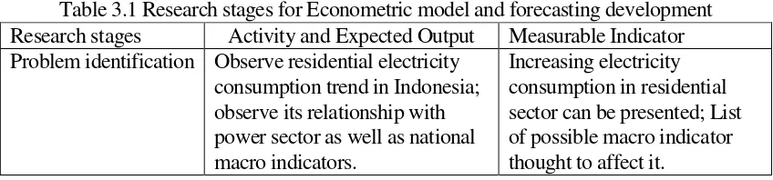
Table 3.1 Research stages for Econometric model and forecasting development Research stages Activity and Expected Output Measurable Indicator Problem identification Observe residential electricity
consumption trend in Indonesia; observe its relationship with power sector as well as national macro indicators.
Problem definition research target, and type of data
Mathematical model under
Research objective Determine the appropriate model for residential’s electricity consumption, determine the macro indicators that affect electricity consumption in residential sector mostly and forecast all the variables in the future Literature review Collect articles and relevant text
books that have appropriate
Data gathering Collect relevant data from PLN, BPS, Bank Indonesia, IMF as they will be served as final data
Availability of several macro indicators as they were appeared initially in earlier stage and have throughly been evaluated, for 1990-2010. Analysis and Result Develop an econometric model
representing residential result includes R, R square, T, F, DW testing, Correlation test, White
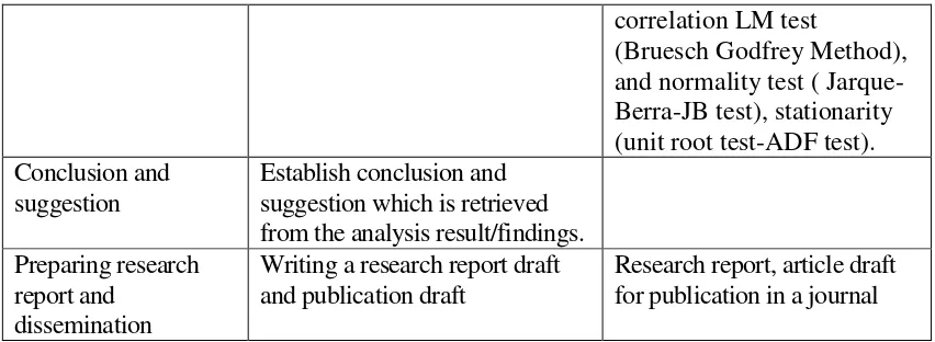
correlation LM test
Table 3.2 Research stages for Factors Decomposition Analysis Research stages Activity and Expected Output Measurable Indicator Problem identification Observe residential electricity
consumption growth in
a certain period of year to be adopted as study period,
Reserach objective Research objectives are proceed through determine appropriate will be selected later as the working method,
establishment of a
decomposition software tool Literature review Reading, observing journal
study further to modified the LMDI and AMDI equation model as the proposed model. Data gathering Collecting relevant data as
required for the purpose of
CHAPTER V
RESULT AND ANALYSIS
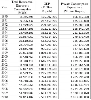
In this chapter, results regarding to residential electricity consumption growth are presented in terms of appropriate annual electricity consumption model and corresponding forecasting model based on econometric method as well as decomposition analysis. Under econometric method, the study period is taken into account 1990 – 2010 whereas for the purpose of decomposition analysis, the study time frame is taken 2000 – 2010. The increasing historical total residential annual electricity consumption growth in Indonesia up to 2010, which is the focus of this research, is presented in below.
Table 5.1. The historical residential annual electricity consumption in Indonesia
1990 8.785.293 195.597.200 106.312.300
1991 9.766.337 227.450.200 125.035.800
1992 11.199.029 259.884.500 135.880.300
1993 12.537.109 302.017.800 158.342.700
1994 14.460.106 382.219.700 221.119.300
1995 16.927.060 454.514.100 279.876.400
1996 19.610.853 532.568.000 325.585.300
1997 22.764.024 627.695.400 387.170.700
1998 24.835.703 955.753.500 647.823.600
1999 26.853.883 1.099.731.600 813.183.300
2000 30.538.269 1.389.769.900 856.798.300
2001 33.318.312 1.646.322.000 1.039.655.000
2002 33.978.744 1.821.833.400 1.231.964.500
2003 35.697.122 2.013.674.600 1.372.078.000
2004 38.579.255 2.295.826.200 1.532.888.300
2005 41.181.839 2.774.281.100 1.785.596.400
2006 43.748.580 3.393.216.800 1.668.718.895
2007 47.321.668 3.950.893.200 1.916.235.454
2008 50.182.040 4.948.688.397 2.234.595.269
2009 54.944.089 5.603.871.170 2.520.631.070
2010 59.823.487 5.501.126.146 2.863.609.098
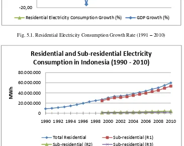
group were classified started on 1998. However, for the purpose of decomposition analysis, the data taken into account started from 1990, which mean require data of 1989 in order to be involved in the calculation. Hence, residential sub-sector electricity consumption shown in the graph is started on 1989.
Fig. 5.1. Residential Electricity Consumption Growth Rate (1991 – 2010)
Fig. 5.2. Total residential and Residential sub-sector Electricity Consumption
As seen on Fig. 5.2., the total residential electricity consumption is primarily contributed by the R1 group, in which the biggest share of residential customer. Here, the main factors to influence electricity consumption in each residential group may not be the same as the consumption growth in fact are different one another.
As residential electricity consumption pattern is observed in two part, i.e. through econometric and decomposition analysis, the total residential electricity consumption model along with its forecasting model are analyze using econometric approach whereas factors to influence for both total residential as well as residential sub-sector are studied using decomposition analysis. Both parts are described belows.
-20,00 -10,00 0,00 10,00 20,00
19911992199319941995199619971998199920002001200220032004200520062007200820092010
Grow
th
(%)
Residential Electricity Consumption Growth
Rate vs GDP Growth Rate in Indonesia
Residential Electricity Consumption Growth (%) GDP Growth (%)
0 20.000.000 40.000.000 60.000.000 80.000.000
1990 1992 1994 1996 1998 2000 2002 2004 2006 2008 2010
MWh
Residential and Sub-residential Electricity
Consumption in Indonesia (1990 - 2010)
Total Residential Sub-residential (R1)
V.1. Econometric Model
The first part of estimation, we constructed a multiple linear model given as:
𝑇𝐸𝐶= 𝛼+ 𝛽1 𝐸𝑚𝑝+ 𝛽2 𝑅𝑒𝑠+𝛽3𝑅𝑒𝑠𝐶𝑢𝑠+ 𝛽4 𝑃𝑜𝑝+ 𝛽5 𝑃𝑟𝑖𝐶𝑜𝑛𝑠+ 𝛽6 𝐸𝑙𝑐𝑡𝑅
+ 𝛽7 𝐵𝐼𝑅𝑎𝑡𝑒+ 𝛽8𝐺𝐷𝑃+ 𝛽9 𝐼𝑛𝑓+ 𝜀
Where:
𝛼 : constanta; 𝛽1 , 𝛽2 , 𝛽3, 𝛽4 , 𝛽5 , 𝛽6 , 𝛽7 , 𝛽8, 𝛽9 : intercepts; 𝜀 : error term
𝑇𝐸𝐶 : Total Energy Consumption
𝐸𝑚𝑝 : Employment
𝑅𝑒𝑠 : Residents
𝑅𝑒𝑠𝐶𝑢𝑠 : Residential Customers
𝑃𝑜𝑝 : Total number of population
𝑃𝑟𝑖𝐶𝑜𝑛𝑠 : Private Consumption 𝐸𝑙𝑐𝑡𝑅 : Electrification ratio 𝐵𝐼𝑅𝑎𝑡𝑒 : Bank Indonesia Rate
𝐺𝐷𝑃 : Total Gross Domestic Product
𝐼𝑛𝑓 : Inflation Rate
The first model was the general model in multiple linear models. Therefore, the next part was to test whether each variables had a problem in least square assumption or known as classical assumption. The first indicator should be tested on each variables was the multicollinearity. As we stated earlier, that the data series should not have a collinearity to each other. If there is a collinearity between the past data and the current data, then this series might not be able as a regressor and the estimation result will not be BLUE (Best Linear Unbiased Estimator).
V.1.1. Correlation Test
To check whether all variables have a multicollinearity problem, we used the correlation test. The results found that employment, total residents, and residential customers have a problem of collinearity. This value of collinearity of those variables are greater than 0.8. Therefore, we cannot use these variables in estimating the model. Meanwhile, the BI rate, Electrification ratio, GDP, Inflation, Population, and Private Consumption had collinearity value less than 0.8. According to these results, we concluded that only BI rate, Electrification ratio. GDP, Inflation, Population, and Private Consumption can be use as regressors in order to estimate the impact on the total energy consumption. The detail results of correlation test are provided in appendix.
V.1.2. White Heteroscedasticity Test
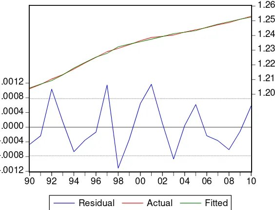
Fig. 5.3. The Actual, Fitted, Residual Graph Result
Figure 5.3. showed that the residual (blue line) is approximately constant and have no trend. This result confirmed us that there is no heteroscedasticity problem occurred in the model. Rather, all variables are homoscedastic.
The second step, we applied White Heteroscedasticity which is provided by Eviews program. The results found that p value observation* 𝑅2 = 0,348489. This p value is greater than 0,05 (95% level of confidence) and we should accept null hypothesis which is no heteroscedasticity. This result also confirmed us that all variables are homoscedastic.
V.1.3. Serial Correlation LM Test
In order to determine whether the variables or regressors have an autocorrelation, we applied two steps. First, we checked t-statistic value, F-value, and Durbin Watson (DW) value particularly. From the estimation result (Table 5.2 below), we found that DW statistic is 1,892522 where is closely to 2 but still less than 2. This result confirmed that the problem of autocorrelation is might not be very significant because the DW statistic is almost 2.
Second, we applied the Serial Correlation LM Test (Bruesch Godfrey Method). The result is p value observation* 𝑅2 = 0,001362. This p value is less than 0,05 (95% level of confidence) and even 0,01. Therefore, we should reject null hypothesis that is no autocorrelation. In conclusion, the model had an autocorrelation problem.
-.0012 -.0008 -.0004 .0000 .0004 .0008 .0012
1.20 1.21 1.22 1.23 1.24 1.25 1.26
90 92 94 96 98 00 02 04 06 08 10
Now we tried to redeem the autocorrelation problem. The first way was to re-construct the model into logarithm normal form. To do so, we changed the form of each variables into logarithm normal form and re-run the estimation testing. After we did the estimation, the result is given in Table 5.2 below. The DW statistic is a little bit higher than before which now is 1,965824. However, the value is still less than 2. The next way was to change the form of regressors into first difference. After we re-estimated and re-runed the first difference model, the result found that, there is no autocorrelation problem.
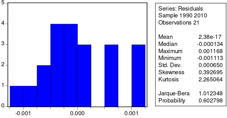
V.1.4. Normality Test
The research had a limitation on data period. We only had 21 observations, which is less than 30 observation (normaly number of observation). Therefore, we applied normality test in order to determine whether the error term is normaly distributed (least square assumption). To do the normality test, we utilized the Jarque-Bera Test and histogram. The result found that p value of Jarque-Bera Test is 0,602798 which is greater than 0,05 (95% level of confidence). Therefore, we cannot reject null hypothesis that is the error term has normaly distributed. In conclusion, the error term of the model is normaly distributed. The result given as seen on Figure 5.4 below:
Fig. 5.4. The Histogram-Normality Test Result
V.1.5. Estimation
After we determined all least square assumptions namely multicollinearity, heteroscedasticity, autocorrelation, and normality, the result confirmed that the research model is relatively become the best estimator in terms of estimating the total energy consumption using a regression method. Therefore, we provide the result of final estimation in Table 5.2 below.
0 1 2 3 4 5
-0.001 0.000 0.001
Series: Residuals Sample 1990 2010 Observations 21
Mean 2.38e-17
Median -0.000134
Maximum 0.001168
Minimum -0.001113
Std. Dev. 0.000650 Skewness 0.392695 Kurtosis 2.265064
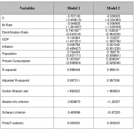
Table 5.2. The estimation results
Adjusted R-squared 0.997211 0.997359
Durbin-Watson stat 1.892522 1.965824
Akaike info criterion -3.838870 -11.22037
Schwarz criterion -3.490696 -10.87220
Prob(F-statistic) 0.000000 0.000000
** Significant at level 0.01 * Siginficant at level 0.05
According to the results, we found that the t-statistic of BI rate, GDP, Inflation, and population are less than 1,96 and the probability of these variables are greater than 0,05 (95% level of significance). These results indicate the acception of null hypotheses which is there is no different between BI rate, GDP, inflation and population to the total energy consumption. We concluded that BI rate, GDP, inflation and population were not significantly affecting the total energy consumption.
However, the R-squared of the model was very high which is 0,998151. It means that the model is the best predictor in estimating the dependent variable. In conclusion, total energy consumption had strongly influenced by the electrification ratio and private consumption. The final equation given as follows:
𝑇𝐸𝐶 = −0,3390−0,0069 𝐵𝐼𝑅𝑎𝑡𝑒+ 0,1582 𝐸𝑙𝑐𝑡𝑅+ 0,1522 𝐺𝐷𝑃+ 0,0010 𝐼𝑛𝑓 + 0,7867 𝑃𝑜𝑝+ 0,2080 𝑃𝑟𝑖𝐶𝑜𝑛
There were several interesting findings from the result equation. First, the coefficient of BI rate showed a negative relationship. It means that if BI rate tends to decrease then total energy consumption will increase. It also confirmed that as a theorethical analysis, BI rate has become a main anchor to analyze the macroeconomic performance. The theory says that when the interest rate tends to fall it will generate high investment including in real sectors. This theory assumed that investors utilize loanable fund from banking system or other financial institutions. In addition, when interest rates decrease then the cost of capital, which is equal to loanable fund, will also tend to decrease. Investors attempt to boost up their investment either in real sector or in financial sector. Furthermore, when the total investment is high, it will also generate new investment in energy contruction in order to expand the energy supply and its capacity. Finally, when the supply of energy increases it will affect the demand for energy to become increase. In terms of supply and demand analysis, when supply getting up the demand also move in the same way in order to keep the price in the same level. Therefore, these concepts are fitted with the research finding. However, BI rate found to be statistically not significant in affecting total energy consumption.
Second, the coefficient of electrification ratio found to be a positive relationship. Since the estimation results confirmed that, the electrification ratio was statistically significant in affecting the total energy consumption, therefore the relationship become more meaningful. The concept stated that the energy consumption would move up as the electrification ratio rose up. The demand for energy occurred when people were realized how important the electricity was in their daily life. When the number of customers increased relatively then it will push up the demand for energy consumption. The result finding was confirmed these concepts particularly.
Third, a positive relationship founded in GDP and total energy consumption. According to the basic concept in consumer behavior, when total income tend to increase then it will moved up the total utility. Satisfaction occurred when the total number of product or services that we consumed is increase. John Maynard Keynes introduced this theory in terms of consumer behavior. GDP is the total income in such a country, which also identify as the total income of people in Indonesia as an aggregate concept. When GDP tend to increase, people will spend their additional income relatively in consumption activity rather than investment. Therefore, the consumption in total energy will tend to increase particularly. However, the result could not statistically confirm that GDP was significant in affecting total energy consumption.
consumption including total energy. Therefore, the expected result was a negative rather than a positive relationship.
Fifth, a positive relationship occurred between number of population and total energy consumption. It was clearly become the expected result regarding the basic theory. It is obvious that additional number of population will cause the shock in total consumption. However, the result could not statistically confirm it.
Sixth, there was a positive relationship between private consumption and total energy consumption. This result also confirmed that households become one of the important parties in macroeconomics point of view. Private consumption is the household’s total consumption in terms of aggregate concept. Other consumptions are investments, government expenditure and international activity such as export and import. In conclusion, the result confirmed that private consumption was statistically significant in affecting the total energy consumption.
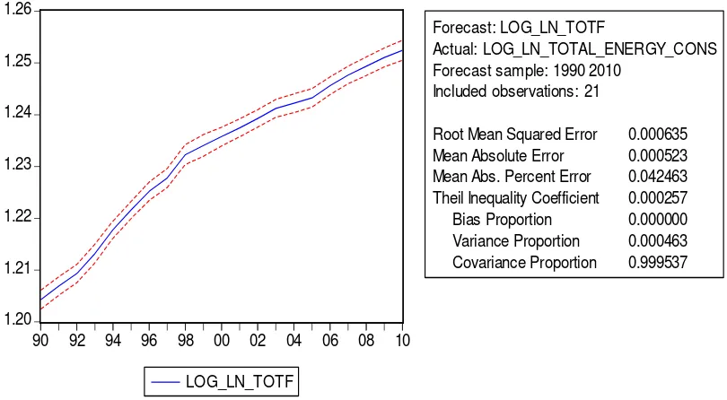
According to the final equation result, we continued to forecast the total energy consumption by using the research period as the sample of forecasting. We can see from Figure 5.5 below, the root mean squared error (RMSE) and theil inequality coefficient are very small which is 0,000635 and 0,000257. It means that the model had a strong power to predict in the future because of the error term are very small. It is one of the purposes of regression method, which is minimizing the error term.
Fig. 5.5. The forecasting result of total energy consumption by using the multiple linear regression model
V.2. Forecasting Model
V.2.1. ARIMA Model
The research used the Box-Jenkins method in order to forecast each variable in the model by itself. In forecasting, first we assumed that all variables could be forecasted by
1.20 1.21 1.22 1.23 1.24 1.25 1.26
90 92 94 96 98 00 02 04 06 08 10
LOG_LN_TOTF
Forecast: LOG_LN_TOTF
Actual: LOG_LN_TOTAL_ENERGY_CONS Forecast sample: 1990 2010
Included observations: 21
other variables not just by the variable itself. The second assumption was the current value of each variable could be affected by the past value of the variable. These two assumption are known as the autoregressive distributed lag model (ADL model). Nevertheless, the paper had a limitation of data observation, which is stated earlier. Therefore, we could not utilize the autoregressive distributed lag model in order to estimate and forecast the total energy consumption. However, we continued to forecast by using the simple Box-Jenkins method that is autoregressive (AR) model, moving average (MA) model, and the integrated and combination of AR and MA model, namely ARIMA model.
First, we constructed the autoregressive (AR) model and moving average (MA) model. In order to construct the model, we had to check the stationarity of each variable by using the unit root test. We applied the Augmented-Dickey Fuller Test to test the stationarity of each variable. The result found that all variables, total energy consumption, electrification ratio, GDP, inflation, population, private consumption, and BI rate are stationary at first difference with trend and intercept (95% level of confidence). These results indicated that we could continue to forecast using the autoregressive dan moving average model.
After we checked the stationarity, then we determined the lag of autoregressive (AR) model by using the correlogram test. The summary of the results given as follows:
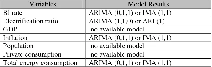
Table 5.3. Summary of ARIMA Model
Variables Model Results
BI rate ARIMA (0,1,1) or IMA (1,1)
Electrification ratio ARIMA (1,1,0) or ARI (1)
GDP no available model
Inflation ARIMA (0,1,1) or IMA (1,1)
Population no available model
Private consumption no available model
Total energy consumption ARIMA (0,1,1) or IMA (1,1)
Table 5.3. showed that the best model in forecasting each variable are choosen from many alternatives models. For example, we found that there are two best alternatives model for inflation. There are ARIMA (1,1,0) and ARIMA (0,1,1). In order to determine which model is the best one, then we should apply the residual test with correlogram Q-statistic to test the autocorrelation. The result was not significant or in other words that there is no autocorrelation. Further, we continued to check the error term by using the Schwarz-Criterion. The smallest value is preferable. The result confirmed that ARIMA (0,1,1) is the best model in forecasting inflation. The similar interpretation is applicable to all variables. The detail results of estimation are provided in appendix.
V.2.2. ARCH/GARCH Model
problem, then we can continue to forecast using the ARCH/GARCH model. According to one of our purposes that are, find the best model in forecasting, therefore we also applied this model into our estimation and forecasting.
First, we had to check the volatility of each variable. This volatility called as the ARCH effect. We used the residual test namely ARCH LM test. If the result found that the variable significantly proved had a volatility or ARCH effect then we continued to estimate the variable using the ARCH model. The summary of the results given as follows:
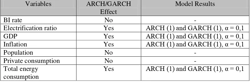
Table 5.4. Summary of ARCH/GARCH Model
Variables ARCH/GARCH
Effect
Model Results
BI rate No -
Electrification ratio Yes ARCH (1) and GARCH (1), α = 0,1
GDP Yes ARCH (1) and GARCH (1), α = 0,1
Inflation Yes ARCH (1) and GARCH (1), α = 0,1
Population No -
Private consumption No -
Total energy consumption
Yes ARCH (1) and GARCH (1), α = 0,1
Table 5.4. showed that electrification ratio, GDP, inflation, and total energy consumption had the ARCH effect and the best model in forecasting are ARCH (1) and GARCH (1) in terms of 10% level of confidence. These results also confirmed that each of variables could affect the variable itself. The detail results are provided in appendix.
V.3. Factors Decomposition for Total Residential Sector
In this section, total residential electricity consumption for 1990 – 2010 is decomposed using AMDI and LMDI methods. The general equation of energy decomposition is given in the appendix. If it is applied for the case of residential electicity consumption decomposition, we should note that the general equation is considered suitable for a system with 100% electrification rate. For the case of Indonesia, of which having less than 100% electrification rate, we modifiy the general equation as:
residential (N), Number of residential customer or electrified household (Nelect), Total residential electricity consumption (Ei), and residential GDP or private expenditure (Yi). The purpose of modifying the general equation is to adjust Residential GDP (Yi) that taken into account both electrified and unelectrified households becomes Adjusted-Yi, which is an approximation value to Adjusted-Yi, obtained from the ratio of Nelect to N multiply with Yi. Fig. 5.3. shows entered and calculated data required for further decomposition process of Indonesia’s residential electricity consumption.
Fig. 5.3. Entered and Calculated Data for Energy Decomposition for Residential Electricity Consumption for AMDI and LMDI methods.
In this research, the AMDI and LMDI analysis are conducted for both additive and multiplicative form. The output given by the tool for both methods are presented in the followings.
Ei Yi adj Yi ei si
2000 1.389.769.900,00 52.008.300,00 26.796.675,00 30.538.269,00 856.798.300,00 441.455.413,57 0,0692 0,3176 2001 1.646.322.000,00 53.560.200,00 27.905.482,00 33.318.312,441.039.655.000,00 541.672.247,09 0,0615 0,3290 2002 1.821.833.400,00 55.041.000,00 28.903.325,00 33.978.744,151.231.964.500,00 646.933.564,65 0,0525 0,3551 2003 2.013.674.600,00 55.623.000,00 29.997.554,00 35.697.121,641.372.078.000,00 739.963.394,59 0,0482 0,3675 2004 2.295.826.200,00 58.253.000,00 31.095.970,00 38.579.255,401.532.888.300,00 818.269.421,15 0,0471 0,3564 2005 2.774.281.100,00 59.927.000,00 32.174.924,00 41.181.838,571.785.596.400,00 958.690.214,17 0,0430 0,3456 2006 3.393.216.800,00 55.942.000,00 33.118.262,00 43.748.579,821.668.718.895,12 987.899.423,92 0,0443 0,2911 2007 3.950.893.200,00 57.006.400,00 34.684.540,00 47.321.668,411.916.235.454,001.165.899.710,45 0,0406 0,2951 2008 4.948.688.397,22 57.716.100,00 36.025.071,00 50.182.040,302.234.595.269,001.394.783.313,88 0,0360 0,2818 2009 5.603.871.170,00 58.421.900,00 37.099.830,00 54.944.088,722.520.631.069,821.600.683.719,34 0,0343 0,2856 2010 5.501.126.146,00 61.363.100,00 39.324.520,00 59.823.486,562.863.609.098,331.835.142.834,37 0,0326 0,3336 Year
Y N Nelect
Decomposition of Energy
Household
∆lnEtot ∆lnEact ∆lnEstr ∆lnEint ∆lnEres Dtot Dact Dstr Dint Dres 2000-2001 0,0871 0,1694 0,0352 -0,1175 0,0000 1,0910 1,1846 1,0358 0,8892 1,0000 2001-2002 0,0196 0,1013 0,0763 -0,1580 0,0000 1,0198 1,1066 1,0793 0,8539 1,0000 2002-2003 0,0493 0,1001 0,0342 -0,0850 0,0000 1,0506 1,1053 1,0348 0,9185 1,0000 2003-2004 0,0776 0,1311 -0,0305 -0,0229 0,0000 1,0807 1,1401 0,9699 0,9773 1,0000 2004-2005 0,0653 0,1893 -0,0309 -0,0931 0,0000 1,0675 1,2084 0,9696 0,9111 1,0000 2005-2006 0,0605 0,2014 -0,1714 0,0304 0,0000 1,0623 1,2231 0,8425 1,0309 1,0000 2006-2007 0,0785 0,1522 0,0135 -0,0872 0,0000 1,0817 1,1644 1,0136 0,9165 1,0000 2007-2008 0,0587 0,2252 -0,0459 -0,1206 0,0000 1,0604 1,2525 0,9551 0,8864 1,0000 2008-2009 0,0907 0,1243 0,0134 -0,0470 0,0000 1,0949 1,1324 1,0134 0,9541 1,0000 2009-2010 0,0851 -0,0185 0,1552 -0,0516 0,0000 1,0888 0,9817 1,1679 0,9497 1,0000 Total 0,6724 1,3758 0,0490 -0,7524 0,0000 10,6978 11,4991 10,0819 9,2876 10,0000
Year
Arithmetic Mean Divisia
Fig. 5.4. Result of AMDI (above) and LMDI (below) result for both additive and multiplicative form.
Using LMDI additive-technique, we find total residential electricity consumption (ΔEtot) in the period 1990 – 2010 became 29.285,2 GWh. The activity effect (ΔEact) which is based GDP changes is the dominant factors contributing electricity consumption growth with 56.634,3 GWh. Insignificant contribution to the increasing electricity consumption was given by the structural effect (ΔEstr), changes in portion of household expenditure to the GDP, with 3.217.9 GWh in aggregate. On the other hand, intensity changes (ΔEint) has consistently shown yearly negative value throughout the study period except for 2005 – 2006. This reveals that the intensity change, which is considered to be due to efficiency improvements, has shown its contribution for a decrease of 30.567 GWh. In multiplicative-LMDI, Dtot, which is the ratio of Et– Et-1 obtained from multiplication of Dact, Dstr, and Dint can be observed without resulting residual variable. The method confirms that the intensity changes is the lowest compared to other changes. Comparison of AMDI and LMDI method in graphical presentation in the period 1990 – 2010 are given in the followings.
∆Etot ∆Eact ∆Estr ∆Eint Dtot Dact Dstr Dint
2000-2001 2.780.043,4400 5.405.409,5772 1.122.481,5352 -3.747.847,6725 1,0910 1,1846 1,0358 0,8892 2001-2002 660.431,7100 3.408.474,6373 2.566.723,2639 -5.314.766,1913 1,0198 1,1066 1,0793 0,8539 2002-2003 1.718.377,4900 3.487.191,8627 1.192.583,0089 -2.961.397,3817 1,0506 1,1053 1,0348 0,9185 2003-2004 2.882.133,7600 4.867.543,6735 -1.133.654,4400 -851.755,4735 1,0807 1,1401 0,9699 0,9773 2004-2005 2.602.583,1700 7.546.662,5314 -1.232.769,5130 -3.711.309,8484 1,0675 1,2084 0,9696 0,9111 2005-2006 2.566.741,2500 8.549.325,3231 -7.275.209,2670 1.292.625,1940 1,0623 1,2231 0,8425 1,0309 2006-2007 3.573.088,5900 6.925.218,0403 614.597,8042 -3.966.727,2545 1,0817 1,1644 1,0136 0,9165 2007-2008 2.860.371,8900 10.974.836,0637 -2.238.768,5652 -5.875.695,6086 1,0604 1,2525 0,9551 0,8864 2008-2009 4.762.048,4200 6.530.959,6333 701.589,7650 -2.470.500,9783 1,0949 1,1324 1,0134 0,9541 2009-2010 4.879.397,8400 -1.061.236,2147 8.900.381,2445 -2.959.747,1898 1,0888 0,9817 1,1679 0,9497 Total 29.285.217,5600 56.634.385,1280 3.217.954,8366 -30.567.122,4045 10,6978 11,4991 10,0819 9,2876
Year
Log-Mean Divisia
Fig. 5.5. Graphical illustration for AMDI and LMDI additive and multiplicative form of Indonesia’s total
residential electricity decomposition
V.4. Factors Decomposition for Residential Sub-sector
R1-residential sub-sector is shown on the figure to represent other sub-sectors in similar manner. Equations to calculate variables for R1 (H1), Yi, ei, s1, s2, s3, and also applies similarly to R2 and R3 are:
, ,
Fig. 5.6. Entered and calculated required data for R1-residential-sub sector decomposition
Outputs given by the tool are determined based on additive and multiplicative form. Fig. 5.7. presents the tool output for R1-residential sub-sector electricity decomposition whereas output calculated for R2 and R3 are included in the appendix.
2000 1.389.769.900,00 30.538.269,00 856.798.300,00 52.008.300,00 26.796.675,00 2001 1.646.322.000,00 33.318.312,44 1.039.655.000,00 53.560.200,00 27.905.482,00 2002 1.821.833.400,00 33.978.744,15 1.231.964.500,00 55.041.000,00 28.903.325,00 2003 2.013.674.600,00 35.697.121,64 1.372.078.000,00 55.623.000,00 29.997.554,00 2004 2.295.826.200,00 38.579.255,40 1.532.888.300,00 58.253.000,00 31.095.970,00 2005 2.774.281.100,00 41.181.838,57 1.785.596.400,00 59.927.000,00 32.174.924,00 2006 3.393.216.800,00 43.748.579,82 1.668.718.895,12 55.942.000,00 33.118.262,00 2007 3.950.893.200,00 47.321.668,41 1.916.235.454,00 57.006.400,00 34.684.540,00 2008 4.948.688.397,22 50.182.040,30 2.234.595.269,00 57.716.100,00 36.025.071,00 2009 5.603.871.170,00 54.944.088,72 2.520.631.069,82 58.421.900,00 37.099.830,00 2010 5.501.126.146,00 59.823.486,56 2.863.609.098,33 61.363.100,00 39.324.520,00
Nelect
Year Ynas E Y N
Ni Ei Yi ei s1 s2 s3
26.484.133,00 28.063.539,00 436.306.515,14 0,0643 0,9883 0,5152 0,6165 27.553.000,00 30.581.615,23 534.830.232,43 0,0572 0,9874 0,5210 0,6315 28.556.684,00 31.161.756,13 639.174.813,79 0,0488 0,9880 0,5251 0,6762 29.629.557,00 32.610.638,86 730.885.844,16 0,0446 0,9877 0,5393 0,6814 30.701.676,00 35.078.627,38 807.893.841,19 0,0434 0,9873 0,5338 0,6677 31.743.229,00 37.325.639,51 945.827.347,05 0,0395 0,9866 0,5369 0,6436 32.660.655,00 39.555.721,49 974.249.260,40 0,0406 0,9862 0,5920 0,4918 34.183.894,00 42.532.237,03 1.149.070.799,74 0,0370 0,9856 0,6084 0,4850 35.482.955,00 45.049.197,03 1.373.794.199,07 0,0328 0,9850 0,6242 0,4516 36.511.814,00 49.298.803,21 1.575.313.585,90 0,0313 0,9842 0,6350 0,4498 38.672.726,00 53.527.188,87 1.804.725.804,77 0,0297 0,9834 0,6408 0,5205
Fig. 5.7. AMDI and LMDI output of R1-residential sub-sector electricity decomposition
In the case of R1-residential sub-sector, ΔEtot is obtained 25.463,6 GWh using LMDI-additive method. If we sum up all residential sub-sector, we will find that ΔEtot is equal to ΔEtot(R1) + ΔEtot(R2) + ΔEtot(R3). However, the changes found in each sub-sector decomposition should not be summed due to reciprocal addition rule. In the case of R1, ΔEtot(R1), which is 25.463,6 GWh is affected by 2 positive changes, i.e. activity changes (ΔEact), obtained for 51.320,9 GWh, and second-term structural changes (ΔEstr2), obtained for 8.558,6 GWh. In other sub-sectors (results included in the appendix), which are R2 and R3, increasing electricity consumption was not only contributed by ΔEstr2, but also by ΔEstr1. It implies that increasing electricity consumption in R1 is indirectly caused by the positive trend of electrified-residential expenditure whereas in R2 and R3, electricity consumption growth are also due to increasing R2 and R3 expenditure, as in the following modified general equations:
,
The residential sub-sectoral additive and multiplicative decomposition for AMDI and LMDI are enclosed in the appendix. Meanwhile, results comparison between two methos are graphically depicted in Fig. 5.8.
∆lnEtot ∆lnEact ∆lnEstr1 ∆lnEstr2 ∆lnEstr3 ∆lnEint ∆lnEres Dtot Dact Dstr1 Dstr2 Dstr3 Dint Dres 2000-2001 0,0859 0,1870 -0,0009 0,0102 0,0221 -0,1081 -0,0244 1,0897 1,1683 0,9991 1,0103 1,0223 0,8976 1,0070 2001-2002 0,0188 0,1635 0,0006 0,0072 0,0628 -0,1463 -0,0690 1,0190 1,0974 1,0006 1,0072 1,0648 0,8639 1,0016 2002-2003 0,0454 0,1227 -0,0003 0,0244 0,0070 -0,0811 -0,0272 1,0465 1,0960 0,9997 1,0247 1,0070 0,9221 1,0039 2003-2004 0,0730 0,0913 -0,0004 -0,0093 -0,0185 -0,0248 0,0347 1,0757 1,1269 0,9996 0,9907 0,9817 0,9755 1,0065 2004-2005 0,0621 0,1431 -0,0007 0,0052 -0,0333 -0,0867 0,0345 1,0641 1,1875 0,9993 1,0053 0,9672 0,9169 1,0057 2005-2006 0,0580 0,0268 -0,0004 0,0885 -0,2436 0,0257 0,1610 1,0597 1,2000 0,9996 1,0925 0,7838 1,0261 1,0055 2006-2007 0,0726 0,1488 -0,0006 0,0247 -0,0125 -0,0834 -0,0045 1,0752 1,1470 0,9994 1,0250 0,9876 0,9200 1,0072 2007-2008 0,0575 0,1604 -0,0006 0,0229 -0,0642 -0,1088 0,0477 1,0592 1,2242 0,9994 1,0232 0,9378 0,8969 1,0059 2008-2009 0,0901 0,1228 -0,0007 0,0155 -0,0035 -0,0419 -0,0020 1,0943 1,1181 0,9993 1,0156 0,9965 0,9589 1,0093 2009-2010 0,0823 0,1218 -0,0007 0,0082 0,1309 -0,0481 -0,1298 1,0858 0,9836 0,9993 1,0082 1,1398 0,9531 1,0086 Total 0,6457 1,2883 -0,0045 0,1975 -0,1529 -0,7035 0,0208 10,6692 11,3489 9,9955 10,2026 9,8885 9,3309 10,0611
Year
Arithmetic Mean Divisia
Additive Multiplicative
∆Etot ∆Eact ∆Estr1 ∆Estr2 ∆Estr3 ∆Eint Dtot Dact Dstr1 Dstr2 Dstr3 Dint
2.518.076,23 4.964.352,09 -28.710,27 326.523,31 704.368,70 -3.448.457,60 1,0897 1,1846 0,9990 1,0112 1,0243 0,8890 580.140,90 3.127.198,85 19.946,17 242.686,80 2.112.224,10 -4.921.915,02 1,0190 1,1066 1,0006 1,0079 1,0708 0,8526 1.448.882,73 3.191.828,36 -8.857,05 849.327,05 242.244,74 -2.825.660,37 1,0465 1,1053 0,9997 1,0270 1,0076 0,9152 2.467.988,52 4.436.132,43 -14.125,50 -346.294,46 -686.883,99 -920.839,96 1,0757 1,1401 0,9996 0,9898 0,9799 0,9731 2.247.012,13 6.850.822,35 -27.033,07 209.094,32 -1.328.196,29 -3.457.675,17 1,0641 1,2084 0,9993 1,0058 0,9640 0,9089 2.230.081,98 7.739.271,23 -15.593,36 3.754.953,55 -10.340.832,05 1.092.282,60 1,0597 1,2231 0,9996 1,1026 0,7641 1,0288 2.976.515,54 6.242.649,23 -25.671,90 1.122.516,06 -568.494,73 -3.794.483,13 1,0752 1,1644 0,9994 1,0277 0,9862 0,9117 2.516.960,00 9.858.117,40 -27.283,53 1.118.476,28 -3.129.444,21 -5.302.905,94 1,0592 1,2525 0,9994 1,0259 0,9310 0,8859 4.249.606,18 5.861.413,87 -38.365,90 812.852,95 -183.189,29 -2.203.105,46 1,0943 1,1324 0,9992 1,0174 0,9961 0,9543 4.228.385,66 -950.851,43 -37.877,10 468.519,23 7.506.086,35 -2.757.491,39 1,0858 0,9817 0,9993 1,0092 1,1573 0,9478 25.463.649,87 51.320.934,39 -203.571,51 8.558.655,08 -5.672.116,66 -28.540.251,44 10,6692 11,4991 9,9950 10,2245 9,8814 9,2673
Log-Mean Divisia
Fig. 5.8. AMDI and LMDI graphical output for R1-electricity consumption decomposition
Dtot Dact Dstr1 Dstr2 Dstr3 Dint Dres
CHAPTER VI
CONCLUSION AND RECOMMENDATION
In this research, econometric model and forecasting model for Indonesia’s electricity consumption growth are constructed and analyzed. In addition, LMDI and AMDI techniques are used to decompose changes in residential electricity consumption in the period 1990 – 2010. Several findings related to the econometric and decomposition analysis in this study are as follows:
1. BI rate, GDP, inflation and population were not significantly affecting the total energy consumption in Indonesia.
2. Electrification ratio and private consumption were significantly affecting to total energy consumption in Indonesia.
3. Total energy consumption had strongly influenced by the electrification ratio and private consumption.
4. The best model through ARIMA model in forecasting BI rate was ARIMA (0,1,1) or IMA (1,1); electrification ratio was ARIMA (1,1,0) or ARI (1); inflation used ARIMA (0,1,1) or IMA (1,1) and total energy consumption utilized ARIMA (0,1,1) or IMA (1,1).
5. The best model through ARCH/GARCH model in forecasting electrification ratio used ARCH (1) and GARCH (1); GDP used ARCH (1) and GARCH (1); Inflation used ARCH (1) and GARCH (1); and total energy consumption used ARCH (1) and GARCH (1).
6. The AMDI method use an arithmetic mean weight function where as the LMDI use a log mean weight function.
7. The LMDI method is preffered than AMDI as using LMDI we can perform perfect decomposition without having residual term, of which accumulates over time in yearly decomposition. In addition, LMDI can work in the case of some available data are zero.
8. Using LMDI additive-technique for the case of total residential sector of Indonesia, we find total residential electricity consumption (ΔEtot) in the period 1990 – 2010 became 29.285,2 GWh. The activity effect (ΔEact) which is based GDP changes is the dominant factors contributing electricity consumption growth with 56.634,3 GWh. Insignificant contribution to the increasing electricity consumption was given by the structural effect (ΔEstr), changes in portion of household expenditure to the GDP, with 3.217.9 GWh in aggregate. On the other hand, intensity changes (ΔEint) has consistently shown yearly negative value throughout the study period except for 2005 – 2006. This reveals that the intensity change, which is considered to be due to efficiency improvements, has shown its contribution for a decrease of 30.567 GWh.
Recommendations
1. According to the result that monetary variables such as Bank Indonesia (BI) rate and inflation rate were not statistically significant in affecting total energy consumption, we recommend to utilize other real sector variables rather than monetary variables in order to analyze the behavior of total energy consumption. In macroeconomics, there is monetary and real sector mechanism of transmission that should be running automatically. However, government and the central bank as the policy makers should be able to analyze the flow of mechanism. Furthermore, they should be achieving macroeconomic final objective that is inflation rate.
2. The result found that the total energy consumption had strongly influenced by the electrification ratio and private consumption, therefore we recommend pushing up the electrification ratio through expanding the electric capacity in Indonesia. This recommendation might be actualize through direct investment in electricity plant and also building a comprehensive infrastructure that can boost up the electrification ratio particularly.
References
Achao, C. and Schaeffer, R. (2009), Decomposition analysis of the variations in residential electricity consumption in Brazil for the 1980-2007 period: Measuring the activity, intensity and structure effects, Energy Policy vol 37 issue 12, pp: 5208-5220, December 2009.
Ang, B.W. (2004), "Decomposition analysis for policymaking in energy: which is the preferred method?", Energy Policy, vol. 32, no. 9, pp. 1131-1139.
Ang, B.W. and Zhang, F.Q. (2000), "A survey of index decomposition analysis in energy and environmental studies", Energy, vol. 25, no. 12, pp. 1149-1176.
Aydinalp, M. et al (2003). Modelling of residential energy consumption at the national level. International Journal of Energy Research, vol 27 issue 4, pp: 441-453, March, 2003.
Chung, W., et al (2011). A study of residential energy use in Hong Kong by decomposition analysis, 1990-2007. Applied Energy vol 88 issue 12, pp: 5180-5187, December 2011. Companies, 2004.
Enders, W. (2004), Applied Econometric Time Series, Second Edition, John-Wiley & Sons, Inc.
Farebrother, R.W. (1980), The Durbin-Watson test for serial correlation when there is no intercept in the regression. Econometrica vol 48 no. 6, September 1980.
Gujarati, D. (2004), Basic Econometrics Fourth Edition. New York: The McGraw-Hill
Hanke, J.E. and Wichern, D.W. (2005), Business Forecasting, Eighth Edition, Pearson-Prentice Hall
Liu, N. and Ang, B.W. (2007), Factors shaping aggregate energy intensity trend for industry: Energy intensity versus product mix., Energy Economics, vol.29, no.4, pp. 609-635.
Lotz, R. I. and Blignaut, J.N. (2011). South Africa’s electricity consumption: A decompotition analysis, Applied Energy vol 88 issue 12, pp: 4779-4784, December 2011.
Min, J., et al (2010). A high resolution statistical model of residential energy end use characteristics for the United States. Journal of Industrial Ecology. Vol 14 issue 5, pp: 791-807, October 2010.
P.T. PLN (Persero) (2011), 2010 PLN Annual report, Jakarta, 2011.
Pachauri, S and Muller, A. (2008), Regional decomposition of domestic electricity consumption in India: 1980-2005. Procceding of the Annual IAEE Conference, Istanbul, 20 June 2008.
APPENDIX
- Economy
Formula Used in This Research PERIOD
PRIVATE CONSUMPTION EXPENDITURE (MILLION
RUPIAH)
GDP (MILLION RUPIAH)
GDP GROWTH
(%)
BI RATE (%)
INFLATION (%)
Correlation Results
EMPL RES_CUS RESIDENTIAL BI_RATE ELECTR GDP GDP_GR INFL POP PRI_CON TOT_EN_CON
Estimation Results
Dependent Variable: TOTAL_ENERGY_CONSUMPT Method: Least Squares
Variable Coefficient Std. Error t-Statistic Prob.
C -5.707133 14.03572 -0.406615 0.6904
BI_RATE -0.046825 0.036534 -1.281687 0.2208 ELECTRIFICATION_RATIO 0.740182 0.133522 5.543516 0.0001
GDP 0.104364 0.074479 1.401251 0.1829
INFLATION 0.006798 0.014482 0.469427 0.6460 POPULATION 0.734259 0.783484 0.937171 0.3646 PRIVATE_CONSUMPTION 0.187530 0.063815 2.938624 0.0108
R-squared 0.998048 Mean dependent var 17.08156
Adjusted R-squared 0.997211 S.D. dependent var 0.589862 S.E. of regression 0.031149 Akaike info criterion -3.838870 Sum squared resid 0.013584 Schwarz criterion -3.490696
Log likelihood 47.30814 F-statistic 1193.011
Durbin-Watson stat 1.892522 Prob(F-statistic) 0.000000
Dependent Variable: TOTAL_ENERGY_CONS Method: Least Squares
Variable Coefficient Std. Error t-Statistic Prob.
C -0.339025 1.013886 -0.334382 0.7430
BI_RATE -0.006906 0.004515 -1.529439 0.1484 ELECTRIFICATION_R 0.158202 0.026525 5.964230 0.0000
GDP 0.152207 0.096107 1.583736 0.1356
INFLATION 0.001049 0.001164 0.901230 0.3827 POPULATION 0.786775 0.839799 0.936861 0.3647 PRIVATE_CONSUMPTION 0.208004 0.079199 2.626346 0.0199
R-squared 0.998151 Mean dependent var 1.232278
Adjusted R-squared 0.997359 S.D. dependent var 0.015124 S.E. of regression 0.000777 Akaike info criterion -11.22037 Sum squared resid 8.46E-06 Schwarz criterion -10.87220
Log likelihood 124.8139 F-statistic 1259.716
ARIMA Models
Method: Least Squares
Convergence achieved after 3 iterations
Variable Coefficient Std. Error t-Statistic Prob.
C 0.004515 0.002923 1.544372 0.1409
AR(1) 0.697124 0.180636 3.859282 0.0013 R-squared 0.466985 Mean dependent var 0.005119 Adjusted R-squared 0.435632 S.D. dependent var 0.005057 S.E. of regression 0.003799 Akaike info criterion -8.208954 Sum squared resid 0.000245 Schwarz criterion -8.109539 Log likelihood 79.98506 F-statistic 14.89406 Durbin-Watson stat 1.982750 Prob(F-statistic) 0.001258 Inverted AR Roots .70
D(LOG_LN_ELECTRIFICATION_R) = 0.004514879351 + [AR(1)=0.6971241405]
Dependent Variable: BI_RATE Method: Least Squares
Variable Coefficient Std. Error t-Statistic Prob.
C 0.394307 0.015873 24.84080 0.0000
R-squared 0.000000 Mean dependent var 0.394307 Adjusted R-squared 0.000000 S.D. dependent var 0.072741 S.E. of regression 0.072741 Akaike info criterion -2.357380 Sum squared resid 0.105825 Schwarz criterion -2.307641 Log likelihood 25.75249 Durbin-Watson stat 0.862596
.48 .52 .56 .60 .64 .68 .72
92 94 96 98 00 02 04 06 08 10
LOG_LN_ELEF
Forecast: LOG_LN_ELEF
Actual: LOG_LN_ELECTRIFICATION_R Forecast sample: 1990 2010
Adjusted sample: 1992 2010 Included observations: 19
Dependent Variable: D(INFLATION) Method: Least Squares
Convergence achieved after 105 iterations
Variable Coefficient Std. Error t-Statistic Prob. C -0.020024 0.006320 -3.168237 0.0053 MA(1) -1.820582 0.534403 -3.406760 0.0031 R-squared 0.829282 Mean dependent var -0.003640 Adjusted R-squared 0.819797 S.D. dependent var 0.304896 S.E. of regression 0.129429 Akaike info criterion -1.156728 Sum squared resid 0.301534 Schwarz criterion -1.057155 Log likelihood 13.56728 F-statistic 87.43681 Durbin-Watson stat 2.861821 Prob(F-statistic) 0.000000 Inverted MA Roots 1.82
Estimated MA process is noninvertible
D(LOG_LN_INFLATION) = -0.02002449863 + [MA(1)=-1.820582086,INITMA=1991]
Dependent Variable: ELECTRIFICATION_R Method: Least Squares
Variable Coefficient Std. Error t-Statistic Prob.
C 0.583230 0.007145 81.63172 0.0000
R-squared 0.000000 Mean dependent var 0.583230 Adjusted R-squared 0.000000 S.D. dependent var 0.032741 S.E. of regression 0.032741 Akaike info criterion -3.953935 Sum squared resid 0.021439 Schwarz criterion -3.904195 Log likelihood 42.51631 Durbin-Watson stat 0.046332
ARCH/GARCH Model
Dependent Variable: ELECTRIFICATION_R Method: ML - ARCH
Convergence achieved after 26 iterations Variance backcast: ON
GARCH = C(2) + C(3)*RESID(-1)^2 + C(4)*GARCH(-1)
Coefficient Std. Error z-Statistic Prob.
C 0.596791 0.001879 317.6721 0.0000
Variance Equation
C 1.46E-05 8.82E-06 1.649636 0.0990
RESID(-1)^2 1.757682 0.923721 1.902828 0.0571 GARCH(-1) -0.621546 0.149115 -4.168225 0.0000 R-squared -0.180124 Mean dependent var 0.583230 Adjusted R-squared -0.388381 S.D. dependent var 0.032741 S.E. of regression 0.038578 Akaike info criterion -5.508915 Sum squared resid 0.025301 Schwarz criterion -5.309958 Log likelihood 61.84361 Durbin-Watson stat 0.039260
Dependent Variable: TOTAL_ENERGY_CONS Method: ML - ARCH
Convergence achieved after 7 iterations Variance backcast: ON
GARCH = C(9) + C(10)*RESID(-1)^2 + C(11)*GARCH(-1) + C(12) *BI_RATE + C(13)* ELECTRIFICATION_R
Coefficient Std. Error z-Statistic Prob.
C -0.225702 1.053294 -0.214282 0.8303
BI_RATE -0.006631 0.007345 -0.902698 0.3667 ELECTRIFICATION_R 0.152716 0.032096 4.758166 0.0000
GDP 0.168744 0.125529 1.344257 0.1789
INFLATION 0.001088 0.003850 0.282581 0.7775 POPULATION 0.687059 0.868757 0.790852 0.4290 PRIVATE_CONS 0.204834 0.124833 1.640869 0.1008
AR(1) 0.004999 0.862628 0.005795 0.9954
Variance Equation
C 9.04E-08 4.74E-06 0.019057 0.9848
RESID(-1)^2 0.149957 1.174349 0.127693 0.8984 GARCH(-1) 0.599990 3.219071 0.186386 0.8521
BI_RATE 7.34E-07 5.20E-06 0.141237 0.8877
R-squared 0.997814 Mean dependent var 1.233702 Adjusted R-squared 0.994068 S.D. dependent var 0.014000 S.E. of regression 0.001078 Akaike info criterion -10.59006 Sum squared resid 8.14E-06 Schwarz criterion -9.942829
Log likelihood 118.9006 F-statistic 266.3198