■ ■ ■
■ ■
■ ■
Jeroen Janssens
Data
Science
at the
DATA /DATA SCIENCE
Associate Professor in the Department of Applied Physics and Applied Mathematics at Columbia University and Chief Data Scientist at The New York Times
“
This book explains how
This hands-on guide demonstrates how the flexibility of the command linecan help you become a more efficient and productive data scientist. You’ll learn how to combine small, yet powerful, command-line tools to quickly obtain, scrub, explore, and model your data.
To get you started—whether you’re on Windows, OS X, or Linux—author Jeroen Janssens has developed the Data Science Toolbox, an easy-to-install virtual environment packed with over 80 command-line tools.
Discover why the command line is an agile, scalable, and extensible technology. Even if you’re already comfortable processing data with, say, Python or R, you’ll greatly improve your data science workflow by also leveraging the power of the command line.
■ Obtain data from websites, APIs, databases, and spreadsheets ■ Perform scrub operations on text, CSV, HTML/XML, and JSON ■ Explore data, compute descriptive statistics, and create
visualizations
■ Manage your data science workflow
■ Create reusable command-line tools from one-liners and existing Python or R code
■ Parallelize and distribute data-intensive pipelines ■ Model data with dimensionality reduction, clustering,
regression, and classification algorithms
Jeroen Janssens
978-1-491-94785-2
[LSI]
Data Science at the Command Line by Jeroen Janssens
Copyright © 2015 Jeroen H.M. Janssens. All rights reserved.
Printed in the United States of America.
Published by O’Reilly Media, Inc., 1005 Gravenstein Highway North, Sebastopol, CA 95472.
O’Reilly books may be purchased for educational, business, or sales promotional use. Online editions are also available for most titles (http://safaribooksonline.com). For more information, contact our corporate/ institutional sales department: 800-998-9938 or [email protected].
Editors: Mike Loukides, Ann Spencer, and Marie Beaugureau
Production Editor: Matthew Hacker Copyeditor: Kiel Van Horn Proofreader: Jasmine Kwityn
Indexer: Wendy Catalano Interior Designer: David Futato Cover Designer: Ellie Volckhausen Illustrator: Rebecca Demarest
October 2014: First Edition
Revision History for the First Edition 2014-09-23: First Release
See http://oreilly.com/catalog/errata.csp?isbn=9781491947852 for release details.
The O’Reilly logo is a registered trademark of O’Reilly Media, Inc. Data Science at the Command Line, the cover image of a wreathed hornbill, and related trade dress are trademarks of O’Reilly Media, Inc.
Table of Contents
Preface. . . xi
1. Introduction. . . 1
Overview 2
Data Science Is OSEMN 2
Obtaining Data 2
Scrubbing Data 3
Exploring Data 3
Modeling Data 3
Interpreting Data 4
Intermezzo Chapters 4
What Is the Command Line? 4
Why Data Science at the Command Line? 7
The Command Line Is Agile 7
The Command Line Is Augmenting 7
The Command Line Is Scalable 8
The Command Line Is Extensible 8
The Command Line Is Ubiquitous 9
A Real-World Use Case 9
Further Reading 12
2. Getting Started. . . 13
Overview 13
Setting Up Your Data Science Toolbox 13
Step 1: Download and Install VirtualBox 14
Step 2: Download and Install Vagrant 14
Step 3: Download and Start the Data Science Toolbox 15
Step 4: Log In (on Linux and Mac OS X) 16
Step 4: Log In (on Microsoft Windows) 16
Step 5: Shut Down or Start Anew 17
Essential Concepts and Tools 17
The Environment 17
Executing a Command-Line Tool 18
Five Types of Command-Line Tools 20
Combining Command-Line Tools 22
Redirecting Input and Output 23
Working with Files 24
Help! 25
Further Reading 27
3. Obtaining Data. . . 29
Overview 29
Copying Local Files to the Data Science Toolbox 30
Local Version of Data Science Toolbox 30
Remote Version of Data Science Toolbox 30
Decompressing Files 31
Converting Microsoft Excel Spreadsheets 32
Querying Relational Databases 34
Downloading from the Internet 35
Calling Web APIs 37
Further Reading 39
4. Creating Reusable Command-Line Tools. . . 41
Overview 42
Converting One-Liners into Shell Scripts 42
Step 1: Copy and Paste 44
Step 2: Add Permission to Execute 45
Step 3: Define Shebang 46
Step 4: Remove Fixed Input 47
Step 5: Parameterize 47
Step 6: Extend Your PATH 48
Creating Command-Line Tools with Python and R 49
Porting the Shell Script 50
Processing Streaming Data from Standard Input 52
Further Reading 53
5. Scrubbing Data. . . 55
Overview 56
Common Scrub Operations for Plain Text 56
Calling the API 155
Inspecting the Results 155
Conclusion 156
Further Reading 156
10. Conclusion. . . 159
Let’s Recap 159
Three Pieces of Advice 160
Be Patient 160
Be Creative 161
Be Practical 161
Where to Go from Here? 161
APIs 161
Shell Programming 162
Python, R, and SQL 162
Interpreting Data 162
Getting in Touch 162
A. List of Command-Line Tools. . . 165
B. Bibliography. . . 183
Index. . . 187
Preface
Data science is an exciting field to work in. It’s also still very young. Unfortunately, many people, and especially companies, believe that you need new technology in order to tackle the problems posed by data science. However, as this book demon‐ strates, many things can be accomplished by using the command line instead, and sometimes in a much more efficient way.
Around five years ago, during my PhD program, I gradually switched from using Microsoft Windows to GNU/Linux. Because it was a bit scary at first, I started with having both operating systems installed next to each other (known as dual-boot). The urge to switch back and forth between the two faded and at some point I was even tinkering around with Arch Linux, which allows you to build up your own custom operating system from scratch. All you’re given is the command line, and it’s up to you what you want to make of it. Out of necessity I quickly became comfortable using the command line. Eventually, as spare time got more precious, I settled down with a GNU/Linux distribution known as Ubuntu because of its easy-of-use and large com‐ munity. Nevertheless, the command line is still where I’m getting most of my work done.
It actually hasn’t been too long ago that I realized that the command line is not just for installing software, system configuration, and searching files. I started learning
about command-line tools such as cut, sort, and sed. These are examples of
command-line tools that take data as input, do something to it, and print the result. Ubuntu comes with quite a few of them. Once I understood the potential of combin‐ ing these small tools, I was hooked.
After my PhD, when I became a data scientist, I wanted to use this approach to do data science as much as possible. Thanks to a couple of new, open source command-line tools including scrape, jq, and json2csv, I was even able to use the command line for tasks such as scraping websites and processing lots of JSON data. In Septem‐ ber 2013, I decided to write a blog post titled “Seven Command-Line Tools for Data Science.” To my surprise, the blog post got quite a bit of attention and I received a lot
of suggestions of other command-line tools. I started wondering whether I could turn this blog post into a book. I’m pleased that, some 10 months later, with the help of many talented people (see the “Acknowledgments” on page 16 below), I was able to do just that.
I’m sharing this personal story not so much because I think you should know how this book came about, but more because I want you to know that I had to learn about the command line as well. Because the command line is so different from using a graphical user interface, it can be intimidating at first. But if I can learn it, then you can as well. No matter what your current operating system is and no matter how you currently do data science, by the end of this book you will be able to also leverage the power of the command line. If you’re already familiar with the command line, or even if you’re already dreaming in shell scripts, chances are that you’ll still discover a few interesting tricks or command-line tools to use for your next data science project.
What to Expect from This Book
In this book, we’re going to obtain, scrub, explore, and model data—a lot of it. This book is not so much about how to become better at those data science tasks. There are already great resources available that discuss, for example, when to apply which stat‐ istical test or how data can be best visualized. Instead, this practical book aims to make you more efficient and more productive by teaching you how to perform those data science tasks at the command line.
While this book discusses over 80 command-line tools, it’s not the tools themselves that matter most. Some command-line tools have been around for a very long time, while others are fairly new and might eventually be replaced by better ones. There are even command-line tools that are being created as you’re reading this. In the past 10 months, I have discovered many amazing command-line tools. Unfortunately, some of them were discovered too late to be included in the book. In short, command-line tools come and go, and that’s OK.
What matters most are the underlying ideas of working with tools, pipes, and data. Most of the command-line tools do one thing and do it well. This is part of the Unix philosophy, which makes several appearances throughout the book. Once you become familiar with the command line, and learn how to combine command-line tools, you will have developed an invaluable skill—and if you can create new tools, you’ll be a cut above.
How to Read This Book
chapter. For example, in Chapter 9, we make use of parallel, which is discussed extensively in Chapter 8.
Data science is a broad field that intersects with many other fields, such as program‐ ming, data visualization, and machine learning. As a result, this book touches on many interesting topics that unfortunately cannot be discussed at full length. Throughout the book, there are suggestions for additional reading. It’s not required to read this material in order to follow along with the book, but when you are interes‐ ted, you can use turn to these suggested readings as jumping-off points.
Who This Book Is For
This book makes just one assumption about you: that you work with data. It doesn’t matter which programming language or statistical computing environment you’re currently using. The book explains all the necessary concepts from the beginning.
It also doesn’t matter whether your operating system is Microsoft Windows, Mac OS X, or some other form of Unix. The book comes with the Data Science Tool‐ box, which is an easy-to-install virtual environment. It allows you to run the command-line tools and follow along with the code examples in the same environ‐ ment as this book was written. You don’t have to waste time figuring out how to install all the command-line tools and their dependencies.
The book contains some code in Bash, Python, and R, so it’s helpful if you have some programming experience, but it’s by no means required to follow along.
Conventions Used in This Book
The following typographical conventions are used in this book:
Italic
Indicates new terms, URLs, email addresses, filenames, and file extensions.
Constant width
Used for program listings, as well as within paragraphs to refer to program ele‐ ments such as variable or function names, databases, data types, environment variables, statements, and keywords.
Constant width bold
Shows commands or other text that should be typed literally by the user.
Constant width italic
Shows text that should be replaced with user-supplied values or by values deter‐ mined by context.
This element signifies a tip or suggestion.
This element signifies a general note.
This element signifies a warning or caution.
Using Code Examples
Supplemental material (virtual machine, data, scripts, and custom command-line tools, etc.) is available for download at https://github.com/jeroenjanssens/data-science-at-the-command-line.
This book is here to help you get your job done. In general, if example code is offered with this book, you may use it in your programs and documentation. You do not need to contact us for permission unless you’re reproducing a significant portion of the code. For example, writing a program that uses several chunks of code from this book does not require permission. Selling or distributing a CD-ROM of examples from O’Reilly books does require permission. Answering a question by citing this book and quoting example code does not require permission. Incorporating a signifi‐ cant amount of example code from this book into your product’s documentation does require permission.
We appreciate, but do not require, attribution. An attribution usually includes the
title, author, publisher, and ISBN. For example: “Data Science at the Command Line
by Jeroen H.M. Janssens (O’Reilly). Copyright 2015 Jeroen H.M. Janssens, 978-1-491-94785-2.”
Safari® Books Online
Safari Books Online is an on-demand digital library that deliv‐ ers expert content in both book and video form from the world’s leading authors in technology and business.
Technology professionals, software developers, web designers, and business and creative professionals use Safari Books Online as their primary resource for research, problem solving, learning, and certification training.
Safari Books Online offers a range of plans and pricing for enterprise, government, education, and individuals.
Members have access to thousands of books, training videos, and prepublication manuscripts in one fully searchable database from publishers like O’Reilly Media, Prentice Hall Professional, Addison-Wesley Professional, Microsoft Press, Sams, Que, Peachpit Press, Focal Press, Cisco Press, John Wiley & Sons, Syngress, Morgan Kauf‐ mann, IBM Redbooks, Packt, Adobe Press, FT Press, Apress, Manning, New Riders, McGraw-Hill, Jones & Bartlett, Course Technology, and hundreds more. For more information about Safari Books Online, please visit us online.
How to Contact Us
We have a web page for this book, where we list non-code-related errata and addi‐
tional information. You can access this page at:
http://datascienceatthecommandline.com
Any errata related to the code, command-line tools, and virtual machine should be submitted as a ticket through GitHub’s issue tracker at:
https://github.com/jeroenjanssens/data-science-at-the-command-line/issues
Please address comments and questions concerning this book to the publisher:
O’Reilly Media, Inc.
1005 Gravenstein Highway North Sebastopol, CA 95472
800-998-9938 (in the United States or Canada) 707-829-0515 (international or local)
707-829-0104 (fax)
To comment or ask technical questions about this book, send email to bookques‐
For more information about our books, courses, conferences, and news, see our web‐ site at http://www.oreilly.com.
Find us on Facebook: http://facebook.com/oreilly
Follow us on Twitter: http://twitter.com/oreillymedia
Watch us on YouTube: http://www.youtube.com/oreillymedia
Follow Jeroen on Twitter: @jeroenhjanssens
Acknowledgments
First of all, I’d like to thank Mike Dewar and Mike Loukides for believing that my blog post, “Seven Command-Line Tools for Data Science,” which I wrote in Septem‐ ber 2013, could be expanded into a book. I thank Jared Lander for inviting me to speak at the New York Open Statistical Programming Meetup, because the prepara‐ tions gave me the idea for writing the blog post in the first place.
Special thanks to my technical reviewers Mike Dewar, Brian Eoff, and Shane Reustle for reading various drafts, meticulously testing all the commands, and providing invaluable feedback. Your efforts have improved the book greatly. The remaining errors are entirely my own responsibility.
I had the privilege of working together with four amazing editors, namely: Ann Spencer, Julie Steele, Marie Beaugureau, and Matt Hacker. Thank you for your guid‐ ance and for being such great liaisons with the many talented people at O’Reilly. Those people include: Huguette Barriere, Sophia DeMartini, Dan Fauxsmith, Yas‐ mina Greco, Rachel James, Jasmine Kwityn, Ben Lorica, Mike Loukides, Andrew Odewahn, and Christopher Pappas. There are many others whom I haven’t met yet because they are operating behind the scenes. Together they ensured that working with O’Reilly has truly been a pleasure.
This book discusses over 80 command-line tools. Needless to say, without these tools, this book wouldn’t have existed in the first place. I’m therefore extremely grateful to all the authors who created and contributed to these tools. The complete list of authors is unfortunately too long to include here; they are mentioned in Appendix A. Thanks especially to Aaron Crow, Jehiah Czebotar, Christopher Groskopf, Dima Kogan, Sergey Lisitsyn, Francisco J. Martin, and Ole Tange for providing help with their amazing command-line tools.
for developing the Data Science Toolbox in the first place; his book Mining the Social Web (O’Reilly) also offers a virtual machine.
Eric Postma and Jaap van den Herik, who supervised me during my PhD program, deserve a special thank you. Over the course of five years they have taught me many lessons. Although writing a technical book is quite different from writing a PhD the‐ sis, many of those lessons proved to be very helpful in the past 10 months as well.
Finally, I’d like to thank my colleagues at YPlan, my friends, my family, and especially my wife, Esther, for supporting me and for disconnecting me from the command line at just the right times.
1The development of the UNIX operating system started back in 1969. It featured a command line since the beginning, and the important concept of pipes was added in 1973.
CHAPTER 1
Introduction
This book is about doing data science at the command line. Our aim is to make you a more efficient and productive data scientist by teaching you how to leverage the power of the command line.
Having both the terms “data science” and “command line” in the title requires an explanation. How can a technology that’s over 40 years old1 be of any use to a field that’s only a few years young?
Today, data scientists can choose from an overwhelming collection of exciting tech‐ nologies and programming languages. Python, R, Hadoop, Julia, Pig, Hive, and Spark are but a few examples. You may already have experience in one or more of these. If so, then why should you still care about the command line for doing data science? What does the command line have to offer that these other technologies and pro‐ gramming languages do not?
These are all valid questions. This first chapter will answer these questions as follows. First, we provide a practical definition of data science that will act as the backbone of this book. Second, we’ll list five important advantages of the command line. Third, we demonstrate the power and flexibility of the command line through a real-world use case. By the end of this chapter we hope to have convinced you that the command line is indeed worth learning for doing data science.
Overview
In this chapter, you’ll learn:
• A practical definition of data science
• What the command line is exactly and how you can use it
• Why the command line is a wonderful environment for doing data science
Data Science Is OSEMN
The field of data science is still in its infancy, and as such, there exist various definitions of what it encompasses. Throughout this book we employ a very practical definition by Mason & Wiggins (2010). They define data science according to the fol‐ lowing five steps: (1) obtaining data, (2) scrubbing data, (3) exploring data, (4) mod‐ eling data, and (5) interpreting data. Together, these steps form the OSEMN model
(which is pronounced as awesome). This definition serves as the backbone of this
book because each step, (except step 5, interpreting data) has its own chapter. The fol‐ lowing five subsections explain what each step entails.
Although the five steps are discussed in a linear and incremental fashion, in practice it is very common to move back and forth between them or to perform multiple steps at the same time. Doing data science is an iterative and nonlinear process. For example, once you have modeled your data, and you look at the results, you may decide to go back to the scrubbing step to adjust the features of the data set.
Obtaining Data
Without any data, there is little data science you can do. So the first step is to obtain data. Unless you are fortunate enough to already possess data, you may need to do one or more of the following:
• Download data from another location (e.g., a web page or server)
• Query data from a database or API (e.g., MySQL or Twitter) • Extract data from another file (e.g., an HTML file or spreadsheet)
• Generate data yourself (e.g., reading sensors or taking surveys)
Scrubbing Data
It is not uncommon that the obtained data has missing values, inconsistencies, errors, weird characters, or uninteresting columns. In that case, you have to scrub, or clean, the data before you can do anything interesting with it. Common scrubbing opera‐ tions include:
• Filtering lines
• Extracting certain columns
• Replacing values
• Extracting words • Handling missing values
• Converting data from one format to another
While we data scientists love to create exciting data visualizations and insightful mod‐ els (steps 3 and 4), usually much effort goes into obtaining and scrubbing the required data first (steps 1 and 2). In “Data Jujitsu,” DJ Patil states that “80% of the work in any data project is in cleaning the data” (2012). In Chapter 5, we demonstrate how the command line can help accomplish such data scrubbing operations.
Exploring Data
Once you have scrubbed your data, you are ready to explore it. This is where it gets interesting, because here you will get really into your data. In Chapter 7, we show you how the command line can be used to:
• Look at your data.
• Derive statistics from your data. • Create interesting visualizations.
Command-line tools introduced in Chapter 7 include csvstat (Groskopf, 2014),
feedgnuplot (Kogan, 2014), and Rio (Janssens, 2014).
Modeling Data
If you want to explain the data or predict what will happen, you probably want to cre‐ ate a statistical model of your data. Techniques to create a model include clustering, classification, regression, and dimensionality reduction. The command line is not suitable for implementing a new model from scratch. It is, however, very useful to be able to build a model from the command line. In Chapter 9, we will introduce several command-line tools that either build a model locally or employ an API to perform the computation in the cloud.
Interpreting Data
The final and perhaps most important step in the OSEMN model is interpreting data. This step involves:
• Drawing conclusions from your data
• Evaluating what your results mean
• Communicating your result
To be honest, the computer is of little use here, and the command line does not really come into play at this stage. Once you have reached this step, it is up to you. This is the only step in the OSEMN model that does not have its own chapter. Instead, we kindly refer you to Thinking with Data by Max Shron (O’Reilly, 2014).
Intermezzo Chapters
In between the chapters that cover the OSEMN steps, there are three intermezzo chapters. Each intermezzo chapter discusses a more general topic concerning data science, and how the command line is employed for that. These topics are applicable to any step in the data science process.
In Chapter 4, we discuss how to create reusable tools for the command line. These personal tools can come from both long commands that you have typed on the com‐ mand line, or from existing code that you have written in, say, Python or R. Being able to create your own tools allows you to become more efficient and productive.
Because the command line is an interactive environment for doing data science, it can become challenging to keep track of your workflow. In Chapter 6, we demon‐ strate a command-line tool called Drake (Factual, 2014), which allows you to define your data science workflow in terms of tasks and the dependencies between them. This tool increases the reproducibility of your workflow, not only for you but also for your colleagues and peers.
In Chapter 8, we explain how your commands and tools can be sped up by running them in parallel. Using a command-line tool called GNU Parallel (Tange, 2014), we can apply command-line tools to very large data sets and run them on multiple cores and remote machines.
What Is the Command Line?
on Mac OS X and Ubuntu, respectively. Ubuntu is a particular distribution of GNU/ Linux, which we’ll be assuming throughout the book.
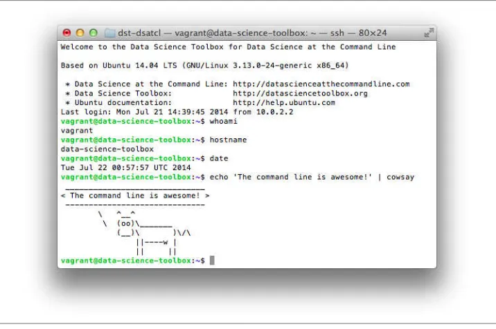
Figure 1-1. Command line on Mac OS X
The window shown in the two screenshots is called the terminal. This is the program that enables you to interact with the shell. It is the shell that executes the commands we type in. (On both Ubuntu and Mac OS X, the default shell is Bash.)
We’re not showing the Microsoft Windows command line (also known as the Command Prompt or PowerShell), because it’s funda‐ mentally different and incompatible with the commands presented in this book. The good news is that you can install the Data Science Toolbox on Microsoft Windows, so that you’re still able to follow along. How to install the Data Science Toolbox is explained in
Chapter 2.
Typing commands is a very different way of interacting with your computer than through a graphical user interface. If you are mostly used to processing data in, say, Microsoft Excel, then this approach may seem intimidating at first. Don’t be afraid. Trust us when we say that you’ll get used to working at the command line very quickly.
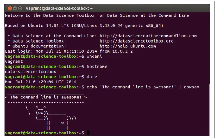
Figure 1-2. Command line on Ubuntu
In this book, the commands that we type in, and the output that they generate, is dis‐ played as text. For example, the contents of the terminal (after the welcome message) in the two screenshots would look like this:
$ whoami
vagrant
$ hostname
data-science-toolbox
$ date
Tue Jul 22 02:52:09 UTC 2014
$ echo 'The command line is awesome!' | cowsay
______________________________ < The command line is awesome! > \ ^__^
\ (oo)\_______ (__)\ )\/\ ||----w | || ||
You’ll also notice that each command is preceded with a dollar sign ($). This is called the prompt. The prompt in the two screenshots showed more information, namely
the username (vagrant), the hostname (data-science-toolbox), and the current
working directory (~). It’s a convention to show only a dollar sign in examples,
directory), (2) can be customized by the user (e.g., it can also show the time or the current git (Torvalds & Hamano, 2014) branch you’re working on), and (3) is irrele‐ vant for the commands themselves.
In the next chapter we’ll explain much more about essential command-line concepts. Now it’s time to first explain why you should learn to use the command line for doing data science.
Why Data Science at the Command Line?
The command line has many great advantages that can really make you a more an efficient and productive data scientist. Roughly grouping the advantages, the com‐ mand line is: agile, augmenting, scalable, extensible, and ubiquitous. We elaborate on each advantage below.
The Command Line Is Agile
The first advantage of the command line is that it allows you to be agile. Data science has a very interactive and exploratory nature, and the environment that you work in needs to allow for that. The command line achieves this by two means.
First, the command line provides a so-called read-eval-print-loop (REPL). This means that you type in a command, press <Enter>, and the command is evaluated immediately. A REPL is often much more convenient for doing data science than the edit-compile-run-debug cycle associated with scripts, large programs, and, say, Hadoop jobs. Your commands are executed immediately, may be stopped at will, and can be changed quickly. This short iteration cycle really allows you to play with your data.
Second, the command line is very close to the filesystem. Because data is the main ingredient for doing data science, it is important to be able to easily work with the files that contain your data set. The command line offers many convenient tools for this.
The Command Line Is Augmenting
Whatever technology your data science workflow currently includes (whether it’s R, IPython, or Hadoop), you should know that we’re not suggesting you abandon that workflow. Instead, the command line is presented here as an augmenting technology that amplifies the technologies you’re currently employing.
The command line integrates well with other technologies. On the one hand, you can often employ the command line from your own environment. Python and R, for instance, allow you to run command-line tools and capture their output. On the other hand, you can turn your code (e.g., a Python or R function that you have
already written) into a command-line tool. We will cover this extensively in Chap‐ ter 4. Moreover, the command line can easily cooperate with various databases and file types such as Microsoft Excel.
In the end, every technology has its advantages and disadvantages (including the command line), so it’s good to know several and use whichever is most appropriate for the task at hand. Sometimes that means using R, sometimes the command line, and sometimes even pen and paper. By the end of this book, you’ll have a solid understanding of when you could use the command line, and when you’re better off continuing with your favorite programming language or statistical computing environment.
The Command Line Is Scalable
Working on the command line is very different from using a graphical user interface (GUI). On the command line you do things by typing, whereas with a GUI, you do things by pointing and clicking with a mouse.
Everything that you type manually on the command line, can also be automated through scripts and tools. This makes it very easy to re-run your commands in case you made a mistake, when the data set changed, or because your colleague wants to perform the same analysis. Moreover, your commands can be run at specific inter‐ vals, on a remote server, and in parallel on many chunks of data (more on that in Chapter 8).
Because the command line is automatable, it becomes scalable and repeatable. It is not straightforward to automate pointing and clicking, which makes a GUI a less suitable environment for doing scalable and repeatable data science.
The Command Line Is Extensible
The command line itself was invented over 40 years ago. Its core functionality has largely remained unchanged, but the tools, which are the workhorses of the command line, are being developed on a daily basis.
The command line itself is language agnostic. This allows the command-line tools to be written in many different programming languages. The open source community is producing many free and high-quality command-line tools that we can use for data science.
The Command Line Is Ubiquitous
Because the command line comes with any Unix-like operating system, including Ubuntu and Mac OS X, it can be found on many computers. According to an article on Top 500 Supercomputer Sites, 95% of the top 500 supercomputers are running GNU/Linux. So, if you ever get your hands on one of those supercomputers (or if you ever find yourself in Jurassic Park with the door locks not working), you better know your way around the command line!
But GNU/Linux doesn’t only run on supercomputers. It also runs on servers, laptops, and embedded systems. These days, many companies offer cloud computing, where you can easily launch new machines on the fly. If you ever log in to such a machine (or a server in general), there’s a good chance that you’ll arrive at the command line.
Besides mentioning that the command line is available in a lot of places, it is also important to note that the command line is not a hype. This technology has been around for more than four decades, and we’re personally convinced that it’s here to stay for another four. Learning how to use the command line (for data science) is therefore a worthwhile investment.
A Real-World Use Case
In the previous sections, we’ve given you a definition of data science and explained to you why the command line can be a great environment for doing data science. Now it’s time to demonstrate the power and flexibility of the command line through a real-world use case. We’ll go pretty fast, so don’t worry if some things don’t make sense yet.
Personally, we never seem to remember when Fashion Week is happening in New York. We know it’s held twice a year, but every time it comes as a surprise! In this
section we’ll consult the wonderful web API of The New York Times to figure out
when it’s being held. Once you have obtained your own API keys on the developer website, you’ll be able to, for example, search for articles, get the list of best sellers, and see a list of events.
The particular API endpoint that we’re going to query is the article search one. We expect that a spike in the amount of coverage in The New York Times about New York Fashion Week indicates whether it’s happening. The results from the API are pagina‐ ted, which means that we have to execute the same query multiple times but with a different page number. (It’s like clicking Next on a search engine.) This is where GNU Parallel (Tange, 2014) comes in handy because it can act as a for loop. The entire command looks as follows (don’t worry about all the command-line arguments given to parallel; we’re going to discuss this in great detail in Chapter 8):
$ cd ~/book/ch01/data
$ parallel -j1 --progress --delay 0.1 --results results "curl -sL "\
> "'http://api.nytimes.com/svc/search/v2/articlesearch.json?q=New+York+'"\
> "'Fashion+Week&begin_date={1}0101&end_date={1}1231&page={2}&api-key='"\
> "'<your-api-key>'" ::: {2009..2013} ::: {0..99} > /dev/null
Computers / CPU cores / Max jobs to run 1:local / 4 / 1
Computer:jobs running/jobs completed/%of started jobs/Average seconds to complete
local:1/9/100%/0.4s
Basically, we’re performing the same query for years 2009-2014. The API only allows up to 100 pages (starting at 0) per query, so we’re generating 100 numbers using brace expansion. These numbers are used by the page parameter in the query. We’re search‐ ing for articles in 2013 that contain the search term New+York+Fashion+Week. Because the API has certain limits, we ensure that there’s only one request at a time, with a one-second delay between them. Make sure that you replace <your-api-key> with your own API key for the article search endpoint.
Each request returns 10 articles, so that’s 1000 articles in total. These are sorted by page views, so this should give us a good estimate of the coverage. The results are in
JSON format, which we store in the results directory. The command-line tool tree
(Baker, 2014) gives an overview of how the subdirectories are structured:
$ tree results | head
results └── 1 ├── 2009 │ └── 2 │ ├── 0
│ │ ├── stderr │ │ └── stdout │ ├── 1
│ │ ├── stderr │ │ └── stdout
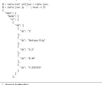
We can combine and process the results using cat (Granlund & Stallman, 2012), jq (Dolan, 2014), and json2csv (Czebotar, 2014):
$ cat results/1/*/2/*/stdout |
> jq -c '.response.docs[] | {date: .pub_date, type: .document_type, '\
> 'title: .headline.main }' | json2csv -p -k date,type,title > fashion.csv Let’s break down this command:
We combine the output of each of the 500 parallel jobs (or API requests).
We convert the JSON data to CSV using json2csv and store it as fashion.csv. With wc -l (Rubin & MacKenzie, 2012), we find out that this data set contains 4,855 articles (and not 5,000 because we probably retrieved everything from 2009):
$ wc -l fashion.csv
4856 fashion.csv
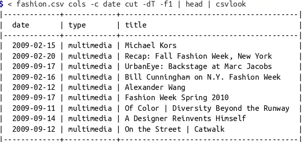
Let’s inspect the first 10 articles to verify that we have succeeded in obtaining the data. Note that we’re applying cols (Janssens, 2014) and cut (Ihnat, MacKenzie, & Meyer‐ ing, 2012) to the date column in order to leave out the time and time zone informa‐ tion in the table: | 2009-09-11 | multimedia | Of Color | Diversity Beyond the Runway | | 2009-09-14 | multimedia | A Designer Reinvents Himself | | 2009-09-12 | multimedia | On the Street | Catwalk | |---+---+---|
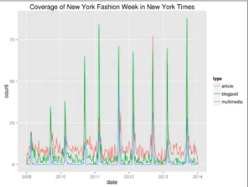
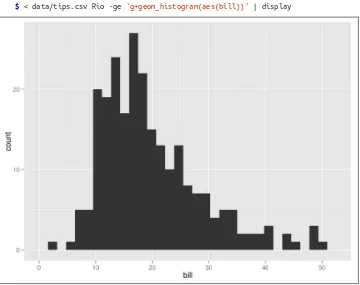
That seems to have worked! In order to gain any insight, we’d better visualize the data. Figure 1-3 contains a line graph created with R (R Foundation for Statistical Comput‐ ing, 2014), Rio (Janssens, 2014), and ggplot2 (Wickham, 2009).
$ < fashion.csv Rio -ge 'g + geom_freqpoly(aes(as.Date(date), color=type), '\
> 'binwidth=7) + scale_x_date() + labs(x="date", title="Coverage of New York'\
> ' Fashion Week in New York Times")' | display
By looking at the line graph, we can infer that New York Fashion Week happens two times per year. And now we know when: once in February and once in September. Let’s hope that it’s going to be the same this year so that we can prepare ourselves! In any case, we hope that with this example, we’ve shown that TheNew York Times API is an interesting source of data. More importantly, we hope that we’ve convinced you that the command line can be a very powerful approach for doing data science.
In this section, we’ve peeked at some important concepts and some exciting command-line tools. Don’t worry if some things don’t make sense yet. Most of the concepts will be discussed in Chapter 2, and in the subsequent chapters we’ll go into more detail for all the command-line tools used in this section.
Figure 1-3. Coverage of New York Fashion Week in The New York Times
Further Reading
• Mason, H., & Wiggins, C. H. (2010). A Taxonomy of Data Science. Retrieved May 10, 2014, from http://www.dataists.com/2010/09/a-taxonomy-of-data-science.
• Patil, D (2012). Data Jujitsu. O’Reilly Media.
• O’Neil, C., & Schutt, R. (2013). Doing Data Science. O’Reilly Media.
CHAPTER 2
Getting Started
In this chapter, we are going to make sure that you have all the prerequisites for doing data science at the command line. The prerequisites fall into two parts: (1) having a proper environment with all the command-line tools that we employ in this book, and (2) understanding the essential concepts that come into play when using the command line.
First, we describe how to install the Data Science Toolbox, which is a virtual environ‐ ment based on GNU/Linux that contains all the necessary command-line tools. Sub‐ sequently, we explain the essential command-line concepts through examples.
By the end of this chapter, you’ll have everything you need in order to continue with the first step of doing data science, namely obtaining data.
Overview
In this chapter, you’ll learn:
• How to set up the Data Science Toolbox
• Essential concepts and tools necessary to do data science at the command line
Setting Up Your Data Science Toolbox
In this book we use many different command-line tools. The distribution of GNU/ Linux that we are using, Ubuntu, comes with a whole bunch of command-line tools pre-installed. Moreover, Ubuntu offers many packages that contain other, relevant command-line tools. Installing these packages yourself is not too difficult. However, we also use command-line tools that are not available as packages and require a more manual, and more involved, installation. In order to acquire the necessary
line tools without having to go through the involved installation process of each, we encourage you to install the Data Science Toolbox.
If you prefer to run the command-line tools natively rather than inside a virtual machine, then you can install the command-line tools individually. However, be aware that this is a very time-consuming process. Appendix A lists all the command-line tools used in the book. The installation instructions are for Ubuntu only, so check the book’s website for up-to-date information on how to install the command-line tools natively on other operating systems. The scripts and data sets used in the book can be obtained by clon‐ ing this book’s GitHub repository.
The Data Science Toolbox is a virtual environment that allows you to get started doing data science in minutes. The default version comes with commonly used soft‐ ware for data science, including the Python scientific stack and R together with its most popular packages. Additional software and data bundles are easily installed. These bundles can be specific to a certain book, course, or organization. You can read more about the Data Science Toolbox at its website.
There are two ways to set up the Data Science Toolbox: (1) installing it locally using VirtualBox and Vagrant or (2) launching it in the cloud using Amazon Web Services. Both ways result in exactly the same environment. In this chapter, we explain how to set up the Data Science Toolbox for Data Science at the Command Line locally. If you wish to run the Data Science Toolbox in the cloud or if you run into problems, refer to the book’s website.
The easiest way to install the Data Science Toolbox is on your local machine. Because the local version of the Data Science Toolbox runs on top of VirtualBox and Vagrant, it can be installed on Linux, Mac OS X, and Microsoft Windows.
Step 1: Download and Install VirtualBox
Browse to the VirtualBox (Oracle, 2014) download page and download the appropri‐ ate binary for your operating system. Open the binary and follow the installation instructions.
Step 2: Download and Install Vagrant
Step 3: Download and Start the Data Science Toolbox
Open a terminal (known as the Command Prompt or PowerShell in Microsoft Win‐ dows). Create a directory, e.g., MyDataScienceToolbox, and navigate to it by typing:
$ mkdir MyDataScienceToolbox
$ cd MyDataScienceToolbox
In order to initialize the Data Science Toolbox, run the following command:
$ vagrant init data-science-toolbox/data-science-at-the-command-line
This creates a file named Vagrantfile. This is a configuration file that tells Vagrant how to launch the virtual machine. This file contains a lot of lines that are commen‐ ted out. A minimal version is shown in Example 2-1.
Example 2-1. Minimal configuration for Vagrant
Vagrant.configure(2) do |config|
config.vm.box = "data-science-toolbox/data-science-at-the-command-line" end
By running the following command, the Data Science Toolbox will be downloaded and booted:
$ vagrant up
If everything went well, then you now have a Data Science Toolbox running on your local machine.
If you ever see the message default: Warning: Connection time out. Retrying... printed repeatedly, then it may be that the vir‐ tual machine is waiting for input. This may happen when the vir‐ tual machine has not been properly shut down. In order to find out what’s wrong, add the following lines to Vagrantfile before the last
end statement (also see Example 2-2):
config.vm.provider "virtualbox"do |vb| vb.gui = true
end
This will cause VirtualBox to show a screen. Once the virtual machine has booted and you have identified the problem, you can remove these lines from Vagrantfile. The username and password to log in are both vagrant. If this doesn’t help, we advise you to check the book’s website, as this website contains an up-to-date list of frequently asked questions.
Example 2-2 shows a slightly more elaborate Vagrantfile. You can view more configu‐ ration options at http://docs.vagrantup.com.
Example 2-2. Configuring Vagrant
Vagrant.require_version ">= 1.5.0"
Vagrant.configure(2) do |config|
config.vm.box = "data-science-toolbox/data-science-at-the-command-line" config.vm.network "forwarded_port", guest: 8000, host: 8000 config.vm.provider "virtualbox" do |vb|
vb.gui = true vb.memory = 2048 vb.cpus = 2 end
end
Require at least version 1.5.0 of Vagrant.
Forward port 8000. This is useful if you want to view a figure you created, as we do in Chapter 7.
Launch a graphical user interface.
Use 2 GB of memory.
Use 2 CPUs.
Step 4: Log In (on Linux and Mac OS X)
If you are running Linux, Mac OS X, or some other Unix-like operating system, you can log in to the Data Science Toolbox by running the following command in a terminal:
$ vagrant ssh
After a few seconds, you will be greeted with the following message:
Welcome to the Data Science Toolbox for Data Science at the Command Line Based on Ubuntu 14.04 LTS (GNU/Linux 3.13.0-24-generic x86_64)
* Data Science at the Command Line: http://datascienceatthecommandline.com * Data Science Toolbox: http://datasciencetoolbox.org
* Ubuntu documentation: http://help.ubuntu.com Last login: Tue Jul 22 19:33:16 2014 from 10.0.2.2
Step 4: Log In (on Microsoft Windows)
recommend PuTTY. Browse to the PuTTY download page and download putty.exe. Run PuTTY, and enter the following values:
• Host Name (or IP address): 127.0.0.1
• Port: 2222
• Connection type: SSH
If you want, you can save these values as a session by clicking the Save button, so that you do not need to enter these values again. Click the Open button and enter vagrant for both the username and the password.
Step 5: Shut Down or Start Anew
The Data Science Toolbox can be shut down by running the following command from the same directory as you ran vagrant up:
$ vagrant halt
In case you wish to get rid of the Data Science Toolbox and start over, you can type:
$ vagrant destroy
Then, return to the instructions for Step 3 to set up the Data Science Toolbox again.
Essential Concepts and Tools
In Chapter 1, we briefly showed you what the command line is. Now that you have your own Data Science Toolbox, we can really get started. In this section, we discuss several concepts and tools that you will need to know in order to feel comfortable doing data science at the command line. If, up to now, you have been mainly working with graphical user interfaces, this might be quite a change. But don’t worry, we’ll start at the beginning, and very gradually go to more advanced topics.
This section is not a complete course in GNU/Linux. We will only explain the concepts and tools that are relevant for doing data sci‐ ence at the command line. One of the advantages of the Data Sci‐ ence Toolbox is that a lot is already set up. If you wish to know more about GNU/Linux, consult “Further Reading” on page 27 at the end of this chapter.
The Environment
So you’ve just logged into a brand new environment. Before we do anything, it’s worthwhile to get a high-level understanding of this environment. The environment is roughly defined by four layers, which we briefly discuss from the top down:
Command-line tools
First and foremost, there are the command-line tools that you work with. We use them by typing their corresponding commands. There are different types of command-line tools, which we will discuss in the next section. Examples of tools are ls (Stallman & MacKenzie, 2012), cat (Granlund & Stallman, 2012), and jq (Dolan, 2014).
Terminal
The terminal, which is the second layer, is the application where we type our commands in. If you see the following text:
$ seq 3
1 2 3
then you would type seq 3 into your terminal and press <Enter>. (The
command-line tool seq (Drepper, 2012) generates a sequence of numbers.) You
do not type the dollar sign. It’s just there to serve as a prompt and let you know that you can type this command. The text below seq 3 is the output of the com‐ mand. In Chapter 1, we showed you two screenshots of how the default terminal looks in Mac OS X and Ubuntu with various commands and their output.
Shell
The third layer is the shell. Once we have typed in our command and pressed <Enter>, the terminal sends that command to the shell. The shell is a program that interprets the command. The Data Science Toolbox uses Bash as the shell, but there are many others available. Once you have become a bit more proficient at the command line, you may want to look into a shell called the Z shell. It offers many additional features that can increase your productivity at the command line.
Operating system
The fourth layer is the operating system, which is GNU/Linux in our case. Linux is the name of the kernel, which is the heart of the operating system. The kernel is in direct contact with the CPU, disks, and other hardware. The kernel also exe‐ cutes our command-line tools. GNU, which is a recursive acronym for GNU’s Not Unix, refers to a set of basic tools. The Data Science Toolbox is based on a particular Linux distribution called Ubuntu.
Executing a Command-Line Tool
$ pwd
/home/vagrant
This is as simple as it gets. You just executed a command that contained a single
command-line tool. The command-line tool pwd (Meyering, 2012) prints the name of
the directory where you currently are. By default, when you log in, this is your home directory. You can view the contents of this directory with ls (Stallman & MacKenzie, 2012):
$ ls
book
The command-line tool cd, which is a Bash builtin, allows you to navigate to a differ‐ ent directory:
The part after cd specifies to which directory you want to navigate to. Values that come after the command are called command-line arguments or options. The two dots refer to the parent directory. Let’s try a different command:
$ head -n 3 data/movies.txt
Matrix Star Wars Home Alone
Here we pass three command-line arguments to head (MacKenzie & Meyering,
2012). The first one is an option. The second one is a value that belongs to the option. The third one is a filename. This particular command outputs the first three lines of the file ~/book/ch02/data/movies.txt.
Sometimes we use commands and pipelines that are too long to fit on the page. In that case, you’ll see something like the following:
$ echo 'Hello'\
> ' world' |
> wc
The greater-than sign (>) is the continuation prompt, which indicates that this line is a continuation of the previous one. A long command can be broken up with either a
backslash (\) or a pipe symbol (|) . Be sure to first match any quotation marks
(" and '). The following command is exactly the same as the previous one:
$ echo 'Hello world' | wc
2Here, we do not refer to the literal Data Science Toolbox we just installed, but to having your own set of tools in a figurative sense.
Five Types of Command-Line Tools
We employ the term “command-line tool” a lot, but we have not yet explained what we actually mean by it. We use it as an umbrella term for anything that can be exe‐ cuted from the command line. Under the hood, each command-line tool is one of the following five types:
• A binary executable
• A shell builtin
• An interpreted script
• A shell function • An alias
It’s good to know the difference between the types. The command-line tools that come pre-installed with the Data Science Toolbox mostly comprise the first two types (binary executable and shell builtin). The other three types (interpreted script, shell function, and alias) allow us to further build up our own data science toolbox2 and become more efficient and more productive data scientists.
Binary executable
Binary executables are programs in the classical sense. A binary executable is cre‐ ated by compiling source code to machine code. This means that when you open the file in a text editor you cannot read its source code.
Shell builtin
Shell builtins are command-line tools provided by the shell, which is Bash in our case. Examples include cd and help. These cannot be changed. Shell builtins may differ between shells. Like binary executables, they cannot be easily inspected or changed.
Interpreted script
An interpreted script is a text file that is executed by a binary executable. Exam‐ ples include: Python, R, and Bash scripts. One great advantage of an interpreted
script is that you can read and change it. Example 2-3 shows a script named ~/
Example 2-3. Python script that computes the factorial of an integer (~/book/ch02/
This script computes the factorial of the integer that we pass as a command-line argument. It can be invoked from the command line as follows:
$ book/ch02/fac.py 5
120
In Chapter 4, we’ll discuss in great detail how to create reusable command-line tools using interpreted scripts.
Shell function
A shell function is a function that is executed by the shell itself; in our case, it is executed by Bash. They provide similar functionality to a Bash script, but they are usually (though not necessarily) smaller than scripts. They also tend to be
more personal. The following command defines a function called fac, which—
just like the interpreted Python script we just looked at—computes the factorial of the integer we pass as a parameter. It does this by generating a list of numbers using seq, putting those numbers on one line with * as the delimiter using paste (Ihnat & MacKenzie, 2012), and passing this equation into bc (Nelson, 2006), which evaluates it and outputs the result:
$ fac() { (echo 1; seq $1) | paste -s -d\* | bc; }
$ fac 5
120
The file ~/.bashrc, which is a configuration file for Bash, is a good place to define your shell functions so that they are always available.
Alias
Aliases are like macros. If you often find yourself executing a certain command with the same parameters (or a part of it), you can define an alias for this. Aliases are also very useful when you continue to misspell a certain command (see his GitHub profile for a long list of useful aliases). The following commands define two aliases:
$ alias l='ls -1 --group-directories-first'
$ alias moer=more
Now, if you type the following on the command line, the shell will replace each alias it finds with its value:
$ cd ~
$ l
book
Aliases are simpler than shell functions as they don’t allow parameters. The func‐
tion fac could not have been defined using an alias because of the parameter.
Still, aliases allow you to save lots of keystrokes. Like shell functions, aliases are often defined in .bashrc or .bash_aliases configuration files, which are located in your home directory. To see all aliases currently defined, you simply run alias without arguments. Try it, what do you see?
In this book, when it comes to creating new command-line tools, we’ll focus mostly on the last three types: interpreted scripts, shell functions, and aliases. This is because these can easily be changed. The purpose of a command-line tool is to make your life on the command line easier, and to make you a more productive and more efficient data scientist. You can find out the type of a command-line tool with type (which is itself a shell builtin):
l is aliased to `ls -1 --group-directories-first'
As you can see, type returns two command-line tools for pwd. In that case, the first reported command-line tool is used when you type pwd. In the next section, we’ll look at how to combine command-line tools.
Combining Command-Line Tools
from its ability to combine these small yet powerful command-line tools. The most
common way of combining command-line tools is through a so-called pipe. The out‐
put from the first tool is passed to the second tool. There are virtually no limits to this.
Consider, for example, the command-line tool seq, which generates a sequence of
numbers. Let’s generate a sequence of five numbers:
$ seq 5
1 2 3 4 5
The output of a command-line tool is by default passed on to the terminal, which dis‐ plays it on our screen. We can pipe the ouput of seq to a second tool, called grep, which can be used to filter lines. Imagine that we only want to see numbers that con‐ tain a “3.” We can combine seq and grep as follows:
$ seq 30 | grep 3
3 13 23 30
And if we wanted to know how many numbers between 1 and 100 contain a “3”, we can use wc, which is very good at counting things:
$ seq 100 | grep 3 | wc -l
19
The -l option specifies that wc should only output the number of lines. By default it also returns the number of characters and words.
You may start to see that combining command-line tools is a very powerful concept. In the rest of the book, you’ll be introduced to many more tools and the functionality they offer when combining them.
Redirecting Input and Output
We mentioned that, by default, the output of the last command-line tool in the pipe‐ line is outputted to the terminal. You can also save this output to a file. This is called output redirection, and works as follows:
$ cd ~/book/ch02
$ seq 10 > data/ten-numbers
Here, we save the output of the seq tool to a file named ten-numbers in the directory ~/book/ch02/data. If this file does not exist yet, it is created. If this file already did
exist, its contents would have been overwritten. You can also append the output to a file with >>, meaning the output is put after the original contents:
$ echo -n "Hello" > hello-world
$ echo " World" >> hello-world
The tool echo simply outputs the value you specify. The -n option specifies that echo should not output a trailing newline.
Saving the output to a file is useful if you need to store intermediate results (e.g., for continuing with your analysis at a later stage). To use the contents of the file hello-world again, we can use cat (Granlund & Stallman, 2012), which reads a file and prints it:
$ cat hello-world | wc -w
2
(Note that the -w option indicates wc to only count words.) The same result can be achieved with the following notation:
$ < hello-world wc -w
2
This way, you are directly passing the file to the standard input of wc without running an additional process. If the command-line tool also allows files to be specified as command-line arguments, which many do, you can also do the following for wc:
$ wc -w hello-world
2 hello-world
Working with Files
As data scientists, we work with a lot of data, which is often stored in files. It’s impor‐ tant to know how to work with files (and the directories they live in) on the com‐ mand line. Every action that you can do using a graphical user interface, you can do with command-line tools (and much more). In this section, we introduce the most important ones to create, move, copy, rename, and delete files and directories.
You have already seen how we can create new files by redirecting the output with either > or >>. In case you need to move a file to a different directory, you can use mv (Parker, MacKenzie, & Meyering, 2012):
$ mv hello-world data
You can also rename files with mv:
$ cd data
$ mv hello-world old-file
$ rm old-file
In case you want to remove an entire directory with all its contents, specify the -r option, which stands for recursive:
$ rm -r ~/book/ch02/data/old
In case you want to copy a file, use cp (Granlund, MacKenzie, & Meyering, 2012). This is useful for creating backups:
$ cp server.log server.log.bak
You can create directories using mkdir (MacKenzie, 2012):
$ cd data
$ mkdir logs
All of these command-line tools accept the -v option, which stands for verbose, so that they output what’s going on. All but mkdir accept the -i option, which stands for interactive, and causes the tools to ask you for confirmation.
Using the command-line tools to manage your files can be scary at first, because you have no graphical overview of the filesystem to provide immediate feedback.
Help!
As you are finding your way around the command line, it may happen that you need help. Even the most-seasoned Linux users need help at some point. It’s impossible to remember all the different command-line tools and their options. Fortunately, the command line offers severals ways to get help.
Perhaps the most important command to get help is perhaps man (Eaton & Watson,
2014), which is short for manual. It contains information for most command-line
tools. Imagine that we forgot the different options to the tool cat. You can access its man page using:
$ man cat | head -n 20
CAT(1) User Commands CAT(1)
NAME
cat - concatenate files and print on the standard output SYNOPSIS
cat [OPTION]... [FILE]... DESCRIPTION
Concatenate FILE(s), or standard input, to standard output. -A, --show-all
equivalent to -vET
-b, --number-nonblank
number nonempty output lines, overrides -n -e equivalent to -vE
Sometimes you’ll see us use head, fold, or cut at the end of a com‐ mand. This is only to ensure that the output of the command fits on the page; you don’t have to type these. For example, head -n 5
only prints the first five lines, fold wraps long lines to 80 charac‐ ters, and cut -c1-80 trims lines that are longer than 80 characters.
Not every command-line tool has a man page. For shell builtins, such as cd, you need to use the help command-line tool:
$ help cd | head -n 20
cd: cd [-L|[-P [-e]] [-@]] [dir] Change the shell working directory.
Change the current directory to DIR. The default DIR is the value of the HOME shell variable.
The variable CDPATH defines the search path for the directory containing DIR. Alternative directory names in CDPATH are separated by a colon (:). A null directory name is the same as the current directory. If DIR begins with a slash (/), then CDPATH is not used.
If the directory is not found, and the shell option 'cdable_vars' is set, the word is assumed to be a variable name. If that variable has a value, its value is used for DIR.
Options:
-L force symbolic links to be followed: resolve symbolic links in DIR after processing instances of '..'
-P use the physical directory structure without following symbolic links: resolve symbolic links in DIR before processing instances
help also covers other topics of Bash, in case you are interested (try help without command-line arguments for a list of topics).
Newer tools that can be used from the command line often lack a man page as well. In that case, your best bet is to invoke the tool with the -h or --help option. For example:
jq --help
jq - commandline JSON processor [version 1.4] Usage: jq [options] <jq filter> [file...]
how to write jq filters (and why you might want to) see the jq manpage, or the online documentation at http://stedolan.github.com/jq
Specifying the --help option also works for GNU command-line tools, such as cat. However, the corresponding man page often provides more information. If after try‐ ing these three approaches, you’re still stuck, then it’s perfectly acceptable to consult the Internet. In Appendix A, there’s a list of all command-line tools used in this book. Besides how each command-line tool can be installed, it also shows how you can get help.
Further Reading
• Janssens, J. H. M. (2014). Data Science Toolbox. Retrieved May 10, 2014, from http://datasciencetoolbox.org.
• Oracle. (2014). VirtualBox. Retrieved May 10, 2014, from http://virtualbox.org.
• HashiCorp. (2014). Vagrant. Retrieved May 10, 2014, from http://vagrantup.com.
• Heddings, L. (2006). Keyboard Shortcuts for Bash. Retrieved May 10, 2014, from http://www.howtogeek.com/howto/ubuntu/keyboard-shortcuts-for-bash-command-shell-for-ubuntu-debian-suse-redhat-linux-etc.
• Peek, J., Powers, S., O’Reilly, T., & Loukides, M. (2002). Unix Power Tools (3rd Ed.). O’Reilly Media.
CHAPTER 3
Obtaining Data
This chapter deals with the first step of the OSEMN model: obtaining data. After all, without any data, there is not much data science that we can do. We assume that the data that is needed to solve the data science problem at hand already exists at some location in some form. Our goal is to get this data onto your computer (or into your Data Science Toolbox) in a form that we can work with.
According to the Unix philosophy, text is a universal interface. Almost every command-line tool takes text as input, produces text as output, or both. This is the main reason why command-line tools can work so well together. However, as we’ll see, even just text can come in multiple forms.
Data can be obtained in several ways—for example by downloading it from a server, by querying a database, or by connecting to a web API. Sometimes, the data comes in a compressed form or in a binary format such as Microsoft Excel. In this chapter, we
discuss several tools that help tackle this from the command line, including: curl
(Stenberg, 2012), in2csv (Groskopf, 2014), sql2csv (Groskopf, 2014), and tar (Bai‐ ley, Eggert, & Poznyakoff, 2014).
Overview
In this chapter, you’ll learn how to:
• Download data from the Internet
• Query databases
• Connect to web APIs
• Decompress files
• Convert Microsoft Excel spreadsheets into usable data
Copying Local Files to the Data Science Toolbox
A common situation is that you already have the necessary files on your own computer. This section explains how you can get those files onto the local or remote version of the Data Science Toolbox.
Local Version of Data Science Toolbox
We mentioned in Chapter 2 that the local version of the Data Science Toolbox is an isolated virtual environment. Luckily, there is one exception to that: files can be trans‐ fered in and out the Data Science Toolbox. The local directory from which you ran vagrant up (which is the one that contains the file Vagrantfile) is mapped to a direc‐ tory in the Data Science Toolbox. This directory is called /vagrant (note that this is not your home directory). Let’s check the contents of this directory:
$ ls -1 /vagrant
Vagrantfile
If you have a file on your local computer, and you want to apply some command-line tools to it, all you have to do is copy or move the file to that directory. Let’s assume that you have a file called logs.csv on your Desktop. If you are running GNU/Linux or Mac OS X, execute the following command on your operating system (and not inside the Data Science Toolbox) from the directory that contains Vagrantfile:
$ cp ~/Desktop/logs.csv .
And if you’re running Windows, you can run the following on the Command Prompt or PowerShell:
> cd %UserProfile%\Desktop
> copy logs.csv MyDataScienceToolbox\
You may also drag and drop the file into the directory using Windows Explorer.
The file is now located in the directory /vagrant. It’s a good idea to keep your data in a separate directory (here we’re using ~/book/ch03/data, for example). So, after you have copied the file, you can move it by running:
$ mv /vagrant/logs.csv ~/book/ch03/data
Remote Version of Data Science Toolbox
If you are running Linux or Mac OS X, you can use scp (Rinne & Ylonen, 2014),