The Collor Plan in Brazil
Marcel Me´rette,Department of Finance, University of Ottawa
In an overlapping generations equilibrium model, the macroeconomic effects of confis-cation of financial assets as occurred in the Collor Plan are studied by means of numerical simulations. The model is built on many features specific to the Brazilian economy, includ-ing a financial system dominated by banks that offer indexed assets and an uneven distribu-tion of wage income and wealth. The framework permits the analysis of the aggregate and redistributive effects of the Collor Plan in a general equilibrium context. The simulation technique developed in this article generates both stationary equilibrium paths and transi-tionary paths. A temporary confiscation of assets simulation replicates the outcomes of the Collor Plan and thus provides insights as to why this stabilization plan failed. This simulation result, plus those of three other simulation experiments, highlights the difficulties in subduing inflation in an indexed economy when inflation taxes are an important source of revenue for the government. These results suggest the need for fiscal reform to enlarge Brazil’s fiscal base and enhance its tax administration in order to win over inflation once and for all. 2000 Society for Policy Modeling. Published by Elsevier Science Inc.
Key Words: Inflation; Overlapping generations; Numerical simulations.
1. INTRODUCTION
On March 15, 1990, Brazil embarked on an innovative and highly risky stabilization effort, the Collor Plan, named after the
Address correspondence to Dr. Marcel Me´rette, Department of Economics, University of Ottawa, 200 Wilbrod St., Ottawa, Canada, K1N 6N5.
This is a revised version of a previous paper entitled “On the Confiscation of Financial Assets in a Credit Economy: The Collor Plan in Brazil,” Centre de recherche et de´veloppe-ment en e´conomique (C.R.D.E.), Cahier 2492, 1992. For this revision the author thanks Irma Adelman and Jean Mercenier for useful comments, and Eunice Kang for editing assistance. Financial support from SSHRC, government of Canada and the program PARADI which is funded by the Canadian International Development Agency, are ac-knowledged. Hospitality from the Economic Growth Center, Yale University, is also grateful.
Received January 1996; final draft accepted September 1996.
Journal of Policy Modeling22(4):417–452 (2000)
country’s new president and the Plan’s staunch advocate, Fer-nando Collor de Mello. One of the main objectives of the Plan was to tackle once and for all the problem of high inflation, which had plagued the Brazilian economy. The Plan took bold measures such as confiscating 80 percent of all banking assets. Even if today nobody contests the failure of the Plan, there does not yet exist in the economic literature a model that satisfactorily explains this failure, probably because of the complexity of the Plan itself. A full explanation is needed, however, because, in the aftermath of the Plan, an abrupt recession followed, and Brazil is still trying to combat its historically high inflation. Moreover, the lessons from the Collor Plan may be important to remember for future stabilization efforts in Brazil or elsewhere. This paper describes the main characteristics of the Brazilian economy and analyzes the consequences of the Collor Plan within the framework of a computable intertemporal general equilibrium model. An overlap-ping generations structure and the use of money as an intertempo-ral complement to other assets are among the features of the model. A computation technique developed for this paper permits the simulation of the shock and counter-shock intended by the Collor Plan. This and other simulation experiments provide in-sights into the failure of the Plan and suggest a set of requirements for the success of a stabilization plan for Brazil.
In this article, Section 2 examines the motivations behind the Collor Plan and describes the Plan in detail. Section 3 provides an informal explanation of the main issues regarding the Plan and refers to the relevance of an overlapping generations structure. Section 4 sets up the model. Section 5 describes the calibration procedure and defines the steady state equilibrium. Section 6 discusses and analyzes the results of four simulations. Section 7 concludes the analysis.
2. THE COLLOR PLAN
In order to grasp the motivations behind the Collor Plan, it is essential to examine the prevailing economic and political climate in Brazil before the new government under president Collor took office. Later, we will describe the different intricacies of the Plan itself.
2A. The Economic and Political Climate
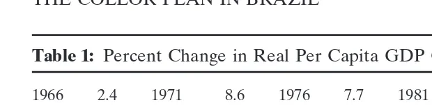
Table 1: Percent Change in Real Per Capita GDP Growth Rate in Brazil
1966 2.4 1971 8.6 1976 7.7 1981 26.5 1986 5.3 1967 1.8 1972 9.3 1977 2.5 1982 21.6 1987 1.5 1968 7.9 1973 11.3 1978 2.6 1983 25.6 1988 22.0 1969 7.1 1974 5.6 1979 4.3 1984 2.7 1989 1.2 1970 5.3 1975 2.7 1980 6.8 1985 5.9 1990–1 23.7
Source:IBGE and Gazeta Mercantil.
was mostly the result of an unprecedented wave of expansion in the world economy that favored Brazilian exports. At the same time, Brazil enjoyed a resurgence in its home economy that culmi-nated in a new influx of investment. This was the “Brazilian mira-cle,” which at its peak (1968–73) featured real per capita annual growth rates over 8 percent (see Table 1). Importing more than 50 percent of its oil needs, Brazil was, nevertheless, able to with-stand the burden of the 1973 oil shock by borrowing profusely on the international market at a favorable rate. The second oil shock of 1979 brought along an altogether different scenario for Brazil. Most industrial countries were confronted with growing inflation and consequently adopted high interest rate policies. On the home front, a rising inflation rate, declining export revenues, high international interest rates, which aggravated the problem of external debt servicing, and the general international pessimism regarding the Brazilian economy triggered a period of hardship for the country throughout the 1980s. In the second half of the 1980s the government of Josey Sarney adopted various stabiliza-tion policies with the hope of resolving, without any social cost,
the joint problem of inflation and a crippled economy.1The overall
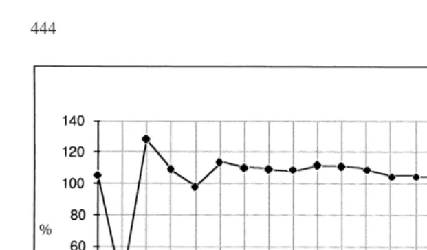
result, which has been dubbed “the lost decade” by Brazilians, was zero (negative) (GDP) growth (per capita) along with perpetually rising inflation rates (see Figure 1).
One of President Collor’s first challenges was thus to prevent an imminent explosion of prices from completely disorganizing the Brazilian economy. Monthly inflation had reached 70 percent when Collor took power (March 14, 1990) and was seriously imper-iling the Brazilian economy. Unlike many other Latin American
1Those plans were called heterodox in the literature because they rely mainly on
Figure 1. Monthly inflation rate in Brazil 1986–1990.
economies, Brazil was not yet prepared to become a dollar econ-omy, because its financial system and centralized, highly regulated labor market offered across-the-board indexation of most financial asset returns and wage prices. The need for indexation of the financial system and the growing risk of dollarization of the econ-omy greatly restrained the scope of monetary policy by forcing the government and the central bank to offer high rates on public titles. Public financing was also in a delicate situation due to a considerable domestic public debt and an operational federal deficit that rose from 5.8 percent of GDP in 1988 to 8.2 percent in 1989. The rise in the federal deficit was ascribed to the wage raise granted to public servants during the final months of the Sarney administration.
• Congressional support for the new government was weak. Collor needed a second round in the presidential elections to obtain the 50 percent of the vote required for his election; it was feared that efforts to negotiate such a plan in Congress would take too much time.
• 1990 was an election year for both Congress and local govern-ments. Collor needed a program that could increase his sup-port within the Congress.
• As Sarney’s government failed in its various attempts to re-store the Brazilian economy, Congress and the public were prepared to accept the drastic solution proposed by Collor.
2B. Measures Undertaken By the Collor Plan
In its economic recovery efforts, the Collor government adopted a series of measures ranging from monetary and fiscal polices to wage and price controls, as well as various external trade policies.
2B-1.Monetary Reform. The most spectacular measures of the
Plan were monetary types. Three drastic policies were immediately adopted:
1. A government’s seizure of 80 percent ofall banking assets,
mostly in the form of a temporary confiscation (18 months) with a smaller proportion taking the form of one-time tax on financial operations.
above a floor level, the burden of this operation was un-equally distributed within the population.
2. A monetary unit change.
The replacement of the old currency, the cruzado novo, by a reincarnated “cruzeiro” served two purposes. First, it permitted the creation of a new government-controlled fi-nancial asset with a nominal value equal to the amount
tem-porarily confiscated. Because this new asset was not tradable,2
it was therefore illiquid. As it was nominated in the previous currency, its rate of return was determined entirely by the government, which promised an annual yield 6 percent higher than that of its treasury bonds. Moreover, it became a liability of the central bank in an accounting twist. Unconfiscated assets were allowed a one-to-one conversion rate from the old currency to the new one. Second, the measure was an attempt to change the inflationary expectations of private agents. As the history of the cruzado novo was associated with the failures of past stabilization plans and a high inflation rate, it was believed that this old currency would render any new stabilization attempts impossible. It was hoped that the simultaneous appearance of a new government and a new currency would modify this.
3. Adoption of a (more) flexible exchange rate.
With a new flexible exchange rate regime, the government had hoped to regain control of the money supply.
The above three measures resulted in the reduction of the
quasi-money stock, M4,3from 33% of GDP to only 8%. The government
felt it would be better to reduce the money stock by too much rather than by too little, mainly because the central bank could no longer rely upon open market operations due to a lack of sufficient demand for government bonds at reasonable rates of return. However, withdrawals in cruzados novos were allowed for the unemployed and retired people, as well for charities, debt, and tax payments. Moreover, most large companies used other loopholes to legally empty their foreign accounts. Consequently, within a few weeks M4 rebounded to 17 percent of GDP.
2The government would not even allow the emergence of a secondary market which
would have made possible the exchange between the old and the new currencies, as suggested by some Brazilian economists. See for instance Carneiro and Goldfajn (1990).
2B-2.Fiscal Policies. The government claimed that the above measures, along with the introduction of the one-time tax on all financial operations, would reverse the operational deficit from an expected 8 percent of GDP to a surplus of 2 percent of GDP. The government also took measures to enlarge its fiscal base by abolishing financial transactions that did not require identification of beneficiaries. Other measures were announced but were not implemented quickly enough to have an influence on the outcome of the Collor Plan. These included privatization of some state companies, a reduction of the public sector, the creation of new taxes and increases in existing ones, the adjustment of public prices
and a reduction in the external debt service.4
2B-3.Wage and Price Policies. Another facet of the
govern-ment’s program was to freeze wages and prices for a period of 30 days. In retrospect, such a measure was somewhat superflu-ous since most inflationary pressures had already been absorbed by the earlier confiscation of financial assets. In subsequent months the government published a list of acceptable price changes, but the scope of these coercive measures was reduced to an increasingly smaller number of items. It was also proposed that wage increases, which were initially under government scru-tiny, should be freely negotiated. In Brazil, however, free collective bargaining in the labor market requires approval from Congress: attempts to muster support for this proposal within Congress were unsuccessful.
2B-4.External Trade. Collor recognized the need for Brazil
to modernize its economy so it could compete on the international market. To achieve this, three measures were announced:
1. The abolition of any quota for imports of machinery, equip-ment and raw materials starting July 1, 1990.
2. The abolition of all administrative controls on imports start-ing July 1, 1990.
3. A gradual reduction in tariffs from average levels of 35 per-cent (ranging between 0 perper-cent and 105 perper-cent) to an average of 20 percent for 1994 (ranging between 0 percent and 40 percent).
4On the slowness of the implementation of these measures, see for instance the Brazilian
However, the government has had considerable difficulties in
implementing these measures.5
3. THE MODELING OF THE BRAZILIAN ECONOMY UNDER THE COLLOR PLAN
As one might now recognize, the Collor Plan was broad and ambitious. Its rationale was that the elimination of the public deficit and repossession of control over the money supply (macro-economic reforms) would defeat inflation while the structural (mi-croeconomic) reforms would place the economy in a new path when their effects were fully felt. The macroeconomic reforms were put in place immediately, while the microeconomic ones were basically left untackled. In this article, we concentrate on the measures actually undertaken. Before setting the model, an informal discussion of the main issues at stake will be helpful. The discussion will attempt to justify the use of an overlapping generations structure in order to study of the Collor Plan.
3A. The Confiscation of Wealth
The confiscation of private wealth, a policy adopted as an infla-tionary remedy in some Latin American countries during the 1980s, has not been discussed much in the literature. It is, neverthe-less, important not to confuse such a measure with the contraction in the money supply flow. It is known that the overall effect of the latter contraction depends largely on the neutrality or super-neutrality of money, as well as whether the policy is anticipated or not. However, the confiscation of private wealth involves other kind of issues:
First, as the confiscation takes the form of seizure of wealth
from private holders, it is a measure that contracts the stock of
money without necessarily modifying monetary policy (theinflux
of money). Second, as was the case for the Collor Plan, the confis-cation policy may also affect wealth accumulated in saving and overnight accounts. In such a case, the confiscation operation leads to a contraction in the amount of quasi-money or credit accumulated by the private agents. This is again a reduction in stock rather than in the flow of private savings. At the seizure
point-in-time, the drop in liquid assets lowers inflationary pres-sures while the drop in accumulated private credit alleviates the burden of public debt services but also crowds out the credit available for working capital. Besides those fundamental distinc-tions, it is crucial in the case of the confiscation of wealth to keep the measure secret until its implementation to avoid any capital
flight from private bank accounts.6In Brazil, promises were made
to investors whose assets were confiscated that the amounts seized would eventually returned. Those promises can do nothing but perplex those whose assets are seized. Thus, a temporary confisca-tion policy as in the Collor Plan introduces immediate contracconfisca-tions as well as future uncertainties.
3B. The Fiscal Consolidation
By converting titles of public debt into new financial assets (the confiscated cruzados novos) and imposing a one-time tax on financial operations, the government hoped to transform an expected 1990 budget deficit into a surplus. But the creation of this new financial asset may rather be an accounting exercise aimed at reducing the officially reported public debt by transferring some liabilities of the national treasury to the central bank. Hence, this
strengthening of public finances may have been illusive.7
More-over, the reduced inflation rate resulting from the Plan no doubt led to a significant decrease in inflation tax revenues, an important source of income for the government. Clearly, the extent of genu-ine fiscal consolidation under such a measure is uncertain as shown in the aftermath of the Plan and in the simulation experiments of this paper, as will be seen below.
3C. The Redistribution of the Tax Burden
Brazil has long had a sophisticated system of indexing returns on financial assets, a system that permits those with high incomes to protect themselves against inflation. A large part of the Brazilian population is excluded from this indexation mechanism simply because it cannot afford to play the financial market. Therefore,
6All banks were closed 5 days before launching the Collor Plan, which implied the
complicity of the preceding Sarney government.
the inflation tax is mostly felt by low and middle class Brazilians.8
By curtailing inflation and seizing some financial assets, the Collor Plan had a redistribution effect benefiting the poor. This helped making the Plan more popular. However, the confiscation of sav-ings soon reduced investment, production and thus the availability of jobs. As a result, the burden of this supposedly progressive tax ended up falling on the lower classes as well. Also, because those with more savings had more assets seized under the Collor Plan, the tax rate implied by the confiscation operation was considered progressive even among investors themselves. These redistribu-tion issues and general equilibrium effects will be consider in the model by the use of an overlapping generations structure.
3D. Why an Overlapping Generations Model?
Hereafter, we will develop a model in which the main features of the Collor Plan’s confiscation are taken into account. We will also perform simulations to analyze the main issues at stake. In this case, an overlapping generations structure is appropriate for several reasons. Overlapping generations model (OLG) is a dy-namic structure within a general equilibrium framework in which agents demand functions are based on microeconomic founda-tions. The OLG have based the agents accumulation of wealth on Modigliani’s life cycle theory: Agents have and dissave at different stages of their life to smooth consumption. The character-istics of the OLG model, that is, its dynamic structure and its allowance for heterogeneous agents, will allow our analysis to take into account the effects of the counter-shock that had been intended by the Collor Plan as well as the reallocation of wealth implied by it among investors. However, the Collor Plan was a stabilization not a structural adjustment plan. Its main objective was short term and consisted of pulling the economy out of a high inflationary path. This is why in the simulations exercises we have chosen quarterly rather than annual data. The question that re-mains is how to integrate the life cycle theory in the Brazilian and Collor Plan context.
Throughout the decade before the launching of the Collor Plan, Brazil has experienced uncertainty together with high inflation rates, checked only temporary by the occasional implementation
8See Cardoso, Barros, and Urani (1993) for the effect of inflation on distribution of
of various economic programs.9 Consequently, Brazilians have
tended to invest in short-run assets, a fact which is compatible with the use of a numerical model based on quarterly data. We can also explain these short-run savings as a preventive measure
against the prospect of job losses,10 illnesses for which costs are
not totally covered by the health system, as well as financial loss
due to crime (theft, assaults, etc.).11 Finally, because few salary
contracts in Brazil provide paid vacations (certainly not those in the black market or the numerous self-employed workers), we may explain investment in short-run assets as a means of financing occasional vacations. We will thus assume that the actions of the representative generation are governed by the life cycle theory, but for only a few quarters at a time. This is not to suggest by any means that Brazilians’ economic behavior is myopic. Rather we believe that the Brazilian experience of years of economic and political turmoil and unstable rates of inflation has rendered any economic calculation a complex adventure and has thus led ordi-nary citizens to plan on a mainly short-run basis.
Uncertainty is the basis for a number of motives invoked to justify the use of the life cycle theory in analyzing the Collor Plan. Most applied general equilibrium models do not explicitly incorporate uncertainty in explaining choices by economic agents. We will not be able to do much better here, except perhaps in accurately reflecting the Brazilian financial planning decision. In our model, each generation will plan its consumption profile on a set period of quarters, the last one being reserved for vacation. More precisely, each generation will work one quarter less than the allowed number of quarters in the consumption plan. The above assumption has two crucial advantages:
1. It captures the short-run nature of Brazilians financial plan-ning.
2. The overlapping structure of the model means that genera-tions differ not by their age but by their financial situation. At each quarter, agents will be at different stages in their
9See Figure 1 again.
10Brazil’s unemployment insurance covers only workers registered with a card, that is
approximately 58 percent of the active population. See Carneiro (1990) on this point.
financial planning and will therefore be affected differently by the confiscation operation.
This overlapping structure thus allows analysis of the redistribu-tion of wealth among the holders of banking assets. Under this assumption, the representative generation does not vanish at the end of a planning period, but merely goes through a new round of planning.
4. THE MODEL
The model of the Brazilian economy in the context of the Collor Plan has two types of consumers, two ways of savings, but only one consumption good. The aggregate output depends on the fixed amount of physical capital and working capital which is predetermined by the amount of credit available for production. The level of credit also determines the demand for labor. The real wage rate of the workers is fixed by Congress and hence there is the possibility of unemployment in the model. Using this model, it will thus be possible to discuss the effect of (reduced) inflation and output of the confiscation operation on various economic agents in the economy.
Any trading between borrowers and lenders must pass through the banking system in this economy. Therefore, one of the main features of the model is the predominance of the banking system as the intermediary financial institution. Credit generated by the banking system is used to produce working capital and to absorb
government domestic debt.12 Banks offer two types of accounts
to investors: a current account that does not protect the investor against an increase in the cost of living, and a savings account that is perfectly indexed to the rate of inflation but requires a minimum deposit. This indivisibility means that an investor who wishes to open or add to any savings deposit must build up his current account beforehand. Therefore, the representative invest-or’s choices must comply with an intertemporal budget constraint containing his consumption, money demand and savings supply. But his choices must also comply with a financial constraint, namely that the money accumulated in this current account (from the previous quarter) is sufficient to acquire a new deposit in his savings account. During the transitional accumulation of money,
the investor pays the inflation tax, which is an important source of income for the government.
The demand for money is derived from a cash-in-advance con-straint. As it serves to finance savings, money will be a complement to other assets in the portfolio. We thus reintegrate an idea first developed by McKinnon (1973) and Shaw (1973) into a dynamic context. Indeed, McKinnon and Shaw show how money becomes a complement to other assets when the banking system is the only intermediary institution. This can be applied to the case of Brazil because the capitalization of all stock exchange markets in Brazil is still less than 25 percent of GDP. In our model however, money
is anintertemporalcomplement to the investor’s savings asset.
A money supply increase serves two purposes. A portion of it finances a fraction of the government budget deficit. Brazil has
frequently relied upon monetization of its deficit.13The magnitude
of this monetization is exogenous in the model. The rest of the money supply is allocated to the private sector in the form of monetary transfers. The rest of the budget deficit is financed through new issues of public debt titles.
We are now ready to set up the model’s structural form. To
avoid confusing notation, we will use indicestfor time period and
gfor the planning stage of the representative generation together
only where necessary. Thereafter, a superscript refers to the stage of the representative generation’s financial plan, and a subscript to the time period in the economy. Lower case letters are for individual quantities, upper case letters for aggregate ones. There are two types of consumers in the model: those with access to the banking system and those without. We will begin with the decision-making problem of the first type of consumers.
4A. The Consumer-Investor Problem
Because consumer–investors have enough income to save and have rational expectations, they must design intertemporal finan-cial plans. It is for these agents that the overlapping generations structure matters. We assume that the representative investor maximizes an intertemporal utility function over a fixed number
of quarters, denoted byG, the last one being unsalaried. At the
13The minister of the economy is a member of the monetary council of the central
end of every financial plan, he repeats the same exercise. We thus
have, at any quarter, G consumer-investors in the economy, all
at various stages in their financial plan. To design a financial plan, the representative investor maximizes a separate logarithmic utility function (Equation 1) with respect to consumption:
Max
cg
o
Gg51
bg21ln(cg). (1)
Now let pg be the money price of the unique consumption
good, ig the nominal rate of return on savings deposits and ikg
the marginal productivity of physical capital. The representative investor is submitted first to a budget constraint. The sum of
consumption expenditurespgcg, money demand (mg2mg21),
sup-ply of savings (pgsg2 pg21sg21) must be less than total income.
Total income is the sum of nominal wage (pgwg), money transfers
received at the end of previous period (trg21), returns on saving
deposits (igpg21sg21), returns on holdings claims on the stock of
Second, the representative investor is submitted to a financial constraint. Here any new savings deposit must be financed by the interest return on the stock accumulated and by money holdings, in his current account, of the previous quarter:
mg211i
g(pg21sg21)>pgsg2pg21sg21. (3)
The above two constraints deserve the following remarks. First, it is assumed that there is no secondary market in the economy. This captures the fact that Brazil is mainly a credit economy. This is why in Equations 2 and 3 there is no term for capital gains on the detention of any asset. Moreover, as will be explained below,
the size of the stocks of physical capitalkand initial government
debtd0held by private agents is exogenously determined by
thin. Indeed, despite its long history of high inflation, Brazil has been able to stay away from any serious dollarization process of the economy. This is somewhat puzzling since many other Latin American countries have been at least partially dollarized. Many factors, including the availability of liquid and indexed banking assets, may explain this observation. Strong legal restrictions on the use of the dollar as a unit of account or means of payments have also limited the size of the parallel dollar market. We assume in this model that legal restrictions reduce dollar demand to zero even if a dollar is a good hedge against the inflation tax.
The equations of the consumer–investor problem are completed by assuming that initial bank deposits and wage income of the
last quarter of the plan are equal to zero (Equation 4).14Moreover,
consumption, money holdings and savings deposits are required to be non-negative (Equation 5).
m050,s050,wG50, (4)
cg>0,mg>0,sg>0. (5)
Given the widespread indexation mechanisms in the Brazilian economy, we adopt the simplifying hypothesis that all rates of return are simultaneously and perfectly indexed to the cost of living. This assumption allows us to rewrite the budget and financial constraints in real terms, and thus to easily insert into Equations
2 and 3 the main object of the discussion, the inflation ratep:
cg1mg1(sg2sg21)<w
In Equation 39the inflation rate equates to the change in nominal
price of the unique consumption good pg 5 (pg/pg21 2 1), mg
is the demand for real money at stageg of the financial plan,rkg
is real rate of return for the claims on capital stock andrgis real
rate of return on debt claims and savings deposits. By Equation
14Because this is a very short-run analysis in which various agents repeat their financial
29, the only tax duty of the representative investor is the inflation
tax. As the real return of money is 1/11 p, the amount of taxes
to be paid is (p/11 p)mg21.
Equations 1, 29, 39, 4, and 5 clearly express the financial problem
faced by the representative investor. With behavior similar to that generated by the life cycle theory, this investor saves to smooth consumption expenditures. The investor has a demand for money since he is submitted to a financial constraint. But in our case,
only the savings good is subject to the financial constraint.15 It
would be unrealistic to include the consumption good in this fi-nancial constraint. Given the persistent high inflation climate, Brazilians do not wait 3 months to spend their cash flow on con-sumption goods.
With this set of constraints, money (or current account
depos-its)16 becomes an intertemporal complement to savings. To see
this, letlgand dgbe the Kuhn–Tucker multipliers for the budget
and the financial constraints, respectively, in the optimization problem of the representative consumer-investor. For interior so-lutions, the first-order conditions of the consumer–investor prob-lem are:
Equation i states, as usual, that the marginal utility of current consumption equals its marginal cost which in turn equals the indirect marginal utility of income. The left-hand side of Equations ii and iii represent the marginal utility of money and savings deposits respectively. These marginal utilities equate the marginal utilities of total and financial incomes for the next period
multiplied by their own rates of return: 1/11 pg11for money and
11rg11for savings deposits. Moreover, using Equation iii for one
quarter ahead and inserting it into Equation ii yields:
15In the literature, consumption or both consumption and savings good are subject to
a financial constraint. See, for instance, Stockman (1981), Abel (1985), and Carmichael (1985, 1987).
16Our definition of money is too narrow to correspond to the Brazilian reality because
11rg12
From this expression we can see that if the investor is ready to sacrifice one unit of current consumption (the right-hand side), he can two quarters later (the left-hand side) receive the sum of the marginal utility of total and financial incomes multiplied by
a rate of return equal to (11rg11)/11 pg11. The presence of the
inflation rate for quarter t 1 1 in the denominator of this ratio
and the presence of the marginal utility of money in the middle of Equation iv neatly illustrate the services of a conduit or inter-temporal complement offered by money in this interinter-temporal substitution experience.
Notice that the presence of two assets in the model does not imply a portfolio effect such as those discussed by Tobin (1969).
On the contrary, the amount of money accumulated at quarterg
complements savings deposits of quarterg11. This is an
intertem-poral way of capturing what has often been observed in undevel-oped and semi-industralized countries.
[I]n the absence of a well-developed equity market, physical capital may be less divisible an asset than in more sophisticated economies. This lumpiness, together with borrowing constraints may make it necessary for investors to accumulate savings for some time in the form of deposits (current account) before investing in physical capital (savings account).17
From this perspective, money serves as a conduit to the formation
of savings.18It is the financial constraint that generates an
intertem-poral complementarity between money and savings in the model. The financial constraint also captures another characteristic of the financial indexation system in Brazil: the indivisibility of savings deposits. It is easy to see, using the life cycle hypothesis, that, for a given intertemporal income and a set of prices and preferences, the longer the operative period without work over a lifetime, the higher the savings rate. In our numerical model, this implies that the average savings ratio depends on the number of quarters included in every round of the financial plan. The smaller this number, the stronger the relative importance of the unsalaried quarter over the entire financial plan and the higher the ratio
17Fry (1988), pp. 22. Italics are ours.
18The housing market is a good example of indivisibility and the complementarity role
Figure 2. Expected profiles for money accumulation and savings deposits.
of savings to wage-income. With the financial constraint, this is consistent with a higher degree of indivisibility for saving deposits. Instead of attributing an arbitrary amount, the degree of indivisi-bility in the model will be captured by the number of quarters
G included in the investor financial plans. This number will be
determined by calibration.
The intertemporal profiles of money demand and savings supply are well defined by the problem of the consumer-investor. To illustrate this, let us successively add up financial constraints for
four quartersG54. This yields the following intertemporal
finan-cial constraint:
(11r4)(11r3) 11 p2
m11(11r4) 11 p3
m21 1 11 p4
m3>s4.
This last expression says that, in order to obtain a planned savings stock for quarter 4, the rate of return will be higher the earlier the money is deposited. For instance, waiting for quarter 3 to execute
the necessary deposit (m3) generates a negative rate of return
will affect investors who are at the beginning of their financial plan, while a savings deposit confiscation affects those who are at the end of their financial plan. Hence in this model, the implied progressiveness of the tax rate and the type of redistribution of wealth between investors will depend upon the type of confiscation.
4B. The Low-Wage Consumer Problem
The Brazilian government claimed that the Collor Plan was progressive by sparing the poor Brazilians an asset confiscation because the majority of them had insufficient revenues to gain access to the indexation system for financial assets in the first place. It is true that the confiscation of wealth did not touch them and this helped to make the operation a popular move at the outset. However, the poor soon suffered as investment and output plummeted. To capture this indirect effect and to better discuss the distribution burden of the Plan, we add to the model agents who consume all of their salary quarter after quarter. These people are “low-wage consumers.” The sum of their consumption level
per quartertis denoted CPt. Let Lt be the total labor employed
at time t, φ the constant share of low-qualified manpower19 and
w˜tthe corresponding wage-income. Then we have:
CPt5w˜tφtLt. (6)
Asφ is fixed, a change in the demand for labor affects low and
highly qualified labor in equal proportions.
4C. The Problem of the Firm
An aggregate Cobb–Douglas function with two aggregate inputs
represents all Brazilian firms. Aggregate outputYdepends on the
fixedKand on working Vcapital stocks:
Yt5AKaV1t2a, (7)
whereAis a scale parameter andathe intensity of fixed physical
capital in the production function. The fixed capital stockK
repre-sents the infrastructure, the factories and large equipment. Be-cause this is a short-term analysis, this stock does not depreciate and is predetermined by history. The consumer–investors and
19Barros et al. (unpublished, 1992) report that almost 50% of income inequality in
government take a constant part of this stock. Even if the volume of this stock is exogenous, it will be helpful in the calibration procedure for the allocation of income between the various eco-nomic agents. Assuming that the national firm takes factor prices as given, first-order conditions from profit maximization push the firm to engage both factors to the point where their physical marginal productivity equal their respective prices.
Working capital at time t, Vt, is assumed to depend on two
intermediate inputs: the credit stock available att21,CRt21, and
the employment level at quartert(orLt). These two intermediate
inputs are connected by a Leontief technology. Denoting the
tech-nological parameter which connects credit and labor byuwe have:
Vt5min(uCRt21,Lt). (8)
In Brazil, real wages are much more an outcome of debates in Congress than of the market. We thus fix the (average) real wage in the model. This assumption together with the hypothesis of a
Leontief technology makes labor employment at timetdependent
on the credit stock available at timet 2 1. Hence, the demand
for labor depends on the accessibility of the t 2 1 credit stock
supplied by the banking system:
Lt5 uCRt21. (9)
Denoting the rate of return on working capital byrvtthe zero profit
condition implies an equality between the revenue generated by the working capital and its cost of production:
rvtVt5wLt1rtCRt21, (10)
wherewis the average wage in the economy.
4D. The Central Bank and the Government
Because Brazil’s central bank is not independent of the govern-ment, both institutions are lumped into one accountable expression. The left-hand side of Equation 11 below represents the expendi-tures minus the incomes of the government, expressed in real terms. Among the expenditure items, real government
consump-tion is denoted byGt, public debt service byrtDt21and real money
transfers by u/1 1 ptMt21. Government income is derived from
returns on the government’s share of fixed physical capital (rkt
KG) and inflation tax revenues by pt/11ptMt21. The government
deficit (right-hand side of the equation) is financed by printing
Gt1rtDt211
Solvency of the government is guaranteed by the satisfaction of the intertemporal budget constraint. To obtain this intertemporal budget constraint, we add up the accountable Equation 11 over
Nperiods. Rearranging somewhat the terms yields:
o
NThe left-hand side of Equation 12 represents the present value of income of the government. The first three terms are seigniorage revenues: the first two are revenues from the increase in real money supply while the third one is from (net) inflation tax. The fourth term of the left-hand side is the present value of income from the ownership’s claim on fixed physical capital. On the right-hand side of Equation 12 there is the present value of government expenditures, the initial stock of debt and the last period of debt and money stocks. If debt and money stocks do not grow as fast or faster than the interest rate on the public debt, the last term on the right-hand side of the Equation 12 converges to zero when
Napproaches infinity. This will happen in the model as long as
the real interest rate is positive since the long-run growth rate of output is zero. This satisfied, the government’s intertemporal budget constraint is reduced to the requirement that the present
value (whenNtends to infinity) of seigniorage and interest returns
on fixed capital must equal the present value of government spend-ing plus the initial stock of government debt:
o
Nthat, in the long run, a necessary condition for the success of any stabilization plan is that the growth rate of government debt and the money supply must not exceed the interest rate on that debt. This constraint restricts feasible fiscal policy options involving changes in revenues and expenditures. For instance, we cannot simulate a permanent increase in government expenditures with-out allowing some time for new taxes to be collected in order to satisfy Equation 13. In case of a temporary change, such as the confiscation of financial assets, the inflation tax revenues must be allowed to change endogenously to comply with Equation 13.
4E. Equilibrium Conditions
Regarding the credit market, the banking system constitutes the unique financial intermediate institution in the economy. To simplify, we assume that the required reserve ratio and the transac-tion and administrative costs of all (private) banks equal zero. As aforementioned, the rate of return on savings deposits offered by banks is perfectly indexed to the cost of living. With perfect competition in the credit market, this rate of return equals the value of the marginal productivity of credit. With the nominal rate of return for money set to zero, profits derived from the inflation tax are entirely and instantaneously dispatched to the
Central Bank.20With all these simplifications, private banks make
no profit. In this model, banks are merely a link between borrowers and lenders. The banks demand savings and lend these to the highest offer between government (under the form of public debt
titles Dt) and firms (under the form of bank credit CRt). The
banks’ activities ensure that the credit market is in equilibrium, where the stock available for production at beginning of quarter
tequals the stock of savings deposits in the banking system, minus
the public debt stock at the end of quartert21:
CRt215
o
G
g51 sg
t212Dt21. (14)
The banks’ portfolios are thus composed of private and public titles which are perfect substitutes. To sell new issues of debt titles, the government must thus offer a rate of return that is marginally higher than the rate on the market until new assets
20This assumption is realistic for Brazil because many banks, including the most
are sold. Notice that from Equation 14, the new public debt titles
at quartert21 crowds out the credit available for production of
quarter t. Moreover, the benchmark data set requires that the
initial stock of public debt be equal to the amount held by all generations in the model:
G·d05D0. (15)
The money market equilibrium condition requires simply that supply equals demand:
Also, the money transfers received by private agents must equal in the aggregate the amount given by the government:
G · trt5uMt. (17)
Fixed capital stock is exogenous and working capital is derived from a predetermined credit supply and the Leontief technology. To maximize profits, firms are always on their demand curves for
both factors of production. Thus, equilibrium conditions for K
andVare also the first-order conditions of national firm’s problem,
which are respectively:
By definition, the fixed capital stock held by the private sector plus that held by the government equals the total stock available in the economy:
G · k1KG5K. (20)
The employment level is derived from the availability of credit
stock of the previous quarter because real wages are fixed.21With
an inelastic labor supply, the unemployment rate mt equals the
difference between labor supply and labor demand:
mt5Ls2Lt. (21)
For accounting purposes, the wage-income of all individuals equals
the wage stock in the economy:
(G21)wt· (12φ)Lt1w˜φLt5wLt. (22)
Finally, the equilibrium condition for the goods market stipu-lates that output equals consumption, plus government expendi-ture and national investment:
Yt5CPt1
o
Gg51 cg
t 1Gt1(CRt2CRt21). (23)
4F. Steady State
In this model, a steady state is a perpetual general equilibrium where all real values are constant and nominal ones grow at a constant rate of inflation. More formally, we have a steady state in this economy when:
1. atomistic (perfect foresight) consumer-investors derive sav-ings supply and demand for the consumption good by the intertemporal optimization of their utility function (Equation
1) subject to the constraints represented by Equations 29, 39,
4, and 5.
2. low-wage consumers derive demand for the consumption good that satisfies Equation 6.
3. the firm, taken as given factor prices, derived their factor demands and output supply from profit maximization, by satisfying Equations 7, 8, 9, and 10.
4. the government budget constraint (Equation 11) is satisfied, as well as the no-Ponzi condition (Equation 13).
5. equilibrium and accounting conditions (Equations 18–23) are satisfied.
6. levels of real flow variables (cg, mg, sg, trg, CP, G) and real
stock variables (V, K, kg,KG,D, M) are constants.
7. wage ratew and rates of returns rk, r, rvare constants.
8. the inflation ratep is constant.
5. CALIBRATING THE MODEL
We calibrate the model after constructing a steady state with the Brazilian data. Non-anticipated shocks are then simulated. For all simulations we are able to resolve numerically for the new
steady state as well as for the path leading up to it.22The method
requires a base solution which is our benchmark steady state. The benchmark steady state data set is generated by using Brazilian macro data from the last quarter in 1988. This is the most recent quarter before the Collor Plan with stable monthly inflation rates. The calibration strategy is mainly to take supply side values of the model from the data and determine demand parameters by satisfying all equilibrium and accountable condi-tions. For instance, we take from the data the inflation rate, the fixed capital stock’s volume and allocation between private and
public sectors,23and the employment level. The capital intensity
parameter for the national firm production function a is taken
from a recent study,24 as are the productivity parameter (wg/w˜)
and the employment share (φ), which distinguish the two types
of consumers.
Once the stocks of both type of capital are known, the scale
parameterA is calibrated by equating GDP at the initial steady
state to one. In this way, all quantities of the initial steady state can be discussed in terms of percentage of GDP. The rates of
return of both capital stocks (rtand rvt) are then easily derived
from the first-order conditions of the firm’s profit maximization
problem. The credit rate of return rt is assumed to equate the
working capital rate of return rvt at the initial steady state. As
can be seen from Equations 8 and 10, this assumption facilitates
the calibration of the average wage rate w. Indeed, given the
employment level,wdepends only on the stock of credit available
in the economy. The level of that stock was determined in the following manner:
With government budget deficit nil in real terms at the steady state, the inflation tax revenues are assumed to be 8 percent of GDP, which was the operational deficit level observed at the beginning of the Collor Plan. Using final quarter data in 1988, the inflation rate was taken to be 105.3 percent—quarterly—and the public debt quarterly GDP ratio was 89.6 percent. The part
22The GAMS-MINOS software is used for the numerical solutions.
23The share was supposed to be identical to the share observed between private and
public investment.
Table 2: Values of the Parameters
Parameters Initial quantities
a A w h wg/w w˜/w φ u G
.4 .0923 .0443 48.8939 1.4 .673 .55 .243 6 Initial prices
p0 rk0 rv0 r0
105.3% 5% 4.52% 4.52%
Initial quantities
M0 D0 G0 L0 V0 K Y ocg
0 CP0 os
g 0
.156 .488 .0946 13.26 13.26 8 1 .688 .217 .2712
of the monetized deficit is assumed to equate the proportion of the public debt that remained out of the hands of private agents, that is 45.5 percent. Given the inflation rate, the money supply
and the money transfer coefficientuare easily determined using
Equation 11 and the monetization coefficient of the deficit. With an intertemporal elasticity of substitution of the utility function
assumed to be one, the number of generationsGis approximated
with the help of first-order conditions and the constraints of the consumer-investors’ problem at a level that ensures that aggregate money demand closely follows money supply which is already
known. The discount factorbis then calibrated to guarantee that
the equilibrium condition for the money market is exactly satisfied. Knowing the generations’ profile of money demand the genera-tions’ profile of savings supply is easily derived (recall Figure 2)
as well as total creditCR0available in the economy. Given CR0
the parameteruof the production function for working capital is
calibrated such that the amount of credit when multiplied by this parameter equals the amount of employment, as required by Equation 9. The fixed average real wage is then derived from the zero profit condition Equation 10. Table 2 summarizes the value of all parameters discussed above. It is worth noting that the various stock-output ratios may look high because the output flow discussed here is based on quarterly data.
6. RESULTS
later, as was initially planned. The second is also a confiscation operation but with no money returned. The third simulation shows how the outcomes depend of the type of asset confiscated. The fourth operates a contraction of government expenditures. The simulations precede over a period of 35 quarters in which the No-Ponzi game condition is set after 20 periods.
6A. The Collor Plan Operation
In the first simulation, the government seizes without warning 10 percent of all bank deposits and 10% of all public debt held
by consumer-investors.25Confiscated money and savings deposits
but not public debt titles are returned to their owners 18 months later in four quarterly and equal installments. This simulation captures all characteristics and issues of the Collor Plan because the shock is operated on stocks rather than on flows, the seizure of initial public debt is tantamount to the one-time tax of the Collor Plan on financial operations, the confiscation of assets is followed by an anticipated monetary counter-shock, and the con-fiscation operation has an uneven character given the presence of two types of consumers and the overlapping structure among the consumer-investors.
All the money and other assets collected go to the Public Trea-sury. Of all assets confiscated (money, savings, and public debt titles), only the seizure of savings assets has an immediate impact on the supply side of the economy by reducing the amount of
credit available to the production of working capitalVt(Equations
8 and 9).26 As the seizure measure seems to have more effect on
the demand side than on the supply side of the economy, the inflation rate is expected to drop. Moreover, with the new revenues collected by the confiscation policy, a government budget surplus is expected assuming everything else as constant. In reality, every-thing else would not be constant. From Equation 11, inflation tax revenues will fall, as well as seigniorage rights from real money demand if the latter drops. A look at Equation 3 raises the possibil-ity of a decline in money demand. Indeed, an unexpected drop in the inflation rate produces a higher rate of return on current accounts, which may lower the demand for money, particularly if the stock of savings desired by the consumer-investors does not increase too much. In other words, the government’s new income
Figure 3. Inflation rate.
derived from its confiscation policy may not compensate the drop in seigniorage revenues.
The government budget balance of quartertaffects output of
the next quarter through the equilibrium condition on the credit market (Equation 14) and through the production functions (Equa-tions 7 and 8). A surplus liberates credit for output and hence contributes to combating inflation, while a deficit generates the exact opposite effect. The results of the simulation, as can be
readily seen in Figures 3 and 4,27suggest a government deficit and
a strong recovery of the inflation rate after a substantial drop. Compared to the initial steady state, the inflation rate drops drastically at first but comes back stronger in the next quarter. This is due to the new government budget deficit (Figure 4) which follows the sharp drop in inflation tax revenues. This drop is not compensated by an increase in real money demand, as can be seen by the evolution of amounts deposited in current accounts (Figure 5). The return of inflation generates more inflation tax revenues and hence a government budget surplus in period 3. Over time, the deficit settles down to its initial level given the imposition of the No Ponzi game condition on government fiscal policy.
27In all figures, quarter 1 corresponds to the initial steady state. We report results up
Figure 4. Government deficit.
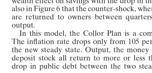
The recession effect is initially strong with a 6 percent drop in GDP. The recession is temporary, due to the unexpected positive wealth effect on savings with the drop in the inflation rate. Notice also in Figure 6 that the counter-shock, when the confiscated assets are returned to owners between quarters 8 and 11, stimulates output.
In this model, the Collor Plan is a complete disaster overall. The inflation rate drops only from 105 percent to 103 percent in the new steady state. Output, the money stock, and the savings deposit stock all return to more or less their initial levels. The drop in public debt between the two steady states is also weak
Figure 6. GDP.
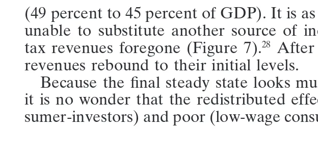
(49 percent to 45 percent of GDP). It is as if the government was unable to substitute another source of income for the inflation
tax revenues foregone (Figure 7).28 After a first drop, these tax
revenues rebound to their initial levels.
Because the final steady state looks much like the initial one, it is no wonder that the redistributed effects between rich (con-sumer-investors) and poor (low-wage consumers) are weak in the
Figure 7. Inflation tax revenue.
28Zini (1992) argues that the Collor Plan II, implemented 10 months after the original
Table 3: Macro Statistics of the Economy of Brazil for Quarters 1990: 2–4
1990:2 1990:3 1990:4
Real deseasonal GDP1 26.56 7.15 22.75
Inflation rate1 32.4 42.5 56.2
Monetary base1 142.7 10.1 76.0
Budget balance2 724.7 782.5 2208.3
Source:IBGE and Conjuntura.
1Percent change relative to previous quarter.
2Million of cruzeiros; include transfers from central bank and the open market
opera-tions on public debt titles.
long run. However, transitional effects are important. For instance, the ratio of consumption levels of the rich versus the poor increase by 15 percent over the first quarter after the plan, thanks to a squeeze in the labor market (employment drops by 10 percent). This, of course, is not what was propagandized by the government. The redistributive effect of this simulation among consumer-inves-tors is also important. For instance, the confiscation has a positive income effect (5.6 percent) on money investors but a negative
one (23.5 percent) on savings investors.
6A-1. Assessing the Accuracy of the Results. The Collor
Plan, at least its stabilization component, died 10 months after being launched when the government, foreseeing the inevitable return of high inflation, froze wages and prices. This new stabiliza-tion plan, called Collor Plan II, also contained measures to syn-chronize the indexation of wages and increase the term of indexed
financial assets.29 Thus, we can compare the results of our first
simulation with only the first three quarters of what we can now call Collor Plan I.
From Table 3, we observe that the drop in GDP and in the inflation rate are similar to those obtained in the simulation. This, of course, may be nothing more than a coincidence. But it is worth noting that GDP recovered in the second quarter of the Plan (1990:3), only to fall again in the following quarter, as occurred in the simulation. While the recovery of the inflation rate was
29This plan was even more short-lived than the first Collor Plan. It died officially only
weaker in reality, the tendency is clear. The resurgence of inflation was spurred by the rise of the monetary base. In this regard, while the target of the central bank was a rise of 14 percent for the second half of 1990, the monetary base actually rose by 93 percent
during that period.30 As the model and the simulation suggest,
this rise can be attributed to the government’s failure to achieve fiscal consolidation since the government budget, even after siz-able transfers from the Central Bank, ended up in deficit for the last quarter of 1990. The surplus in the government budget for 1990:2 is probably a result of a special provision taken by the government which resulted in a temporary but sizable gain in tax collection. This special provision, which allowed debtors to settle fiscal debts with blocking assets, is not captured by the model.
The stock levels obtained in the simulation are also quite accu-rate with reality. Indeed, most wealth stocks did not change much during that period. Between March 1990 and January 1991, M1 drops only from $11.5 to $10.1 billions, but M4 increases from $55 to $59 billions. Because GDP growth averaged out to zero during this period, there is no evidence of portfolio shifts to dollars or gold, as was assumed in the model. Notice, however, that the savings stock (M3) drops from $21.3 to $13.7 billion, a fact that explains the prolonged recession in the aftermath of the Plan.
6B. The Confiscation Operation without Returned Money
Among the most severe concerns expressed over the Collor Plan I was the fear that a strong inflation rate would occur again when the confiscated assets were returned to the owners. We can evaluate the validity of this concern using our model by operating the same confiscation measure as above but excluding any possibil-ity of a future refund. Figure 8 allows the comparison of the inflation rate movement under the modified Plan (the black path) to that of the Collor Plan (the white path). As can be seen, this fear is not justified, the difference between the two appears to be small. This similarity is due to the assumption of forward looking expectations adopted in the model. Indeed, with optimizing and forward looking agents, their behavior changes well before the return of the confiscated assets. In Figure 8, the anticipation of
30The rise cannot be attributed to foreign reserves. The latter increased very little during
Figure 8. Inflation rates comparison.
money refund only marginally increases the inflation rate com-pared to the scenario of no refund.
In June 1992, 24 months after the launching of the Plan, the government returned 65% of the temporarily confiscated cruzados novos, an operation which, as in the model, did not accelerate the inflation rate. The apprehension of an intertemporal debt overhang was thus somewhat exaggerated. In fact, the inflation rate recov-ered much earlier and for other reasons as mentioned above.
6C. The Choice Over Which Asset to Confiscate
Table 4: Assets Variation in Percentage
Public Debt Titles Money Savings
Inflation rate 224.2 212.5 18.6
Public debt 21.1 0.5 21.5
GDP 0 0 22.8
This suggests that any confiscation operation is risky and may yield unpleasant surprises even in the short run.
6D. A Contraction of the Government Expenditures
After the failures of Collor Plan I and II, economic policies changed to a more conventional orientation. To illustrate how a damaging outcome can come out of a meritorious effort, we simulated a 10 percent contraction in government expenditures. The inflation rate at the new steady state ended up just 2.2 percent less than the initial one. The drop in inflation tax revenues is stronger than the contraction of expenditures itself; thus after a drop, inflation comes back stronger as was seen in the Collor Plan simulation. These two experiences suggest that the Brazilian economy, thanks to its sophisticated indexation mechanism, seems difficult to dislodge from the upward bend of the Laffer (inflation tax) curve. If this is indeed the case, a more elaborate fiscal reform program is recommended. An effort to enhance the tax base and streamline tax collection could be more beneficial than anything else in this regard.
7. CONCLUSION
investment in economic activities is threatened. The drop in the savings stocks registered after the Collor Plan indicates that this loss of trust has effectively occurred and may explain the prolonged recession that has followed the Plan.
The existence of an inflation tax Laffer curve might explain why it is easier to combat inflation in a hyperinflation context than in a sophisticated indexed economy such as Brazil’s. Under hyperin-flation, the inflation tax revenue are near zero; any monetary con-traction shock cannot involve a tax revenues squeeze as occurred in this model. In Brazil, as long as inflation tax revenues are not replaced adequately, the reduction in the inflation rate can only be very short-term. After an initial drop, inflation tends to over-shoot its steady state level. This may explain all the failures of Brazil’s stabilization plans throughout the 1980s (recall Figure 1). Based on its continuing endeavor to combat inflation, at least two lessons from the simulations emerge. First, because of the complementarity between money and wealth, a stabilizing fiscal and monetary regime is one that avoids financing a budget by printing money or issuing (short-term) indebtedness titles. Second, within a sophisticated indexation system, the way a budget surplus is generated may be more important than the surplus itself. For instance, finding substitutes for inflation tax revenues may gener-ate more positive outcomes than cutting government expenditures.
REFERENCES
Abel, A. (1985) Dynamic Behavior of Capital Accumulation in a Cash-in-Advance Model.
Journal of Monetary Economics16:55–71.
Cardoso, E.A. (1992) Deficit Finance and Monetary Dynamics in Brazil and Mexico.
Journal of Economics Development37:173–197.
Cardoso, E., Barros, R., and Urani, A. (1993) Inflation and Unemployment as Determinants of Inequality in Brazil: the 1980s. Texto para discussa˜oNo. 298, IPEA, Rio de Janeiro, Brazil.
Carmichael, B. (1985) Anticipated Inflation and the Stock Market.Canadian Journal of EconomicsXVIII(2):285–293.
Carmichael, B. (1987) Cash-in-Advance Economics, Thesis Summary, Mimeo.
Carneiro, D.D. (1990) O Plano Collor: Os Primeiros Tres Meses. Mimeo, Pontefical Universidade Catolica, Rio de Janeiro.
Carneiro, D.D., and Goldfajn, I. (1990) Reforma Monetaria: Pro and Contras do Mercado Secundario. InPlano Collor Avaliacoes e Perpectivas,Livros Tecnicos e Cientificos Editora, 205–223.
Fry, M.J. (1988)Money, Interest, and Banking in Economic Development.Baltimore and London: The Johns Hopkins University Press.
Kotlikoff, L.J. (1989)What Determines Savings?Cambridge: The M.I.T. Press.
Marins Duclos, M.T. (1990) A contribucao do Capital Humano no Crescimento do Brasil: Mensuracao a Analise para as Decadas de 50 a 80. Master Thesis, EPGE, Fundacao Getulio Vargas, Rio de Janeiro.
McKinnon, R.I. (1973)Money and Capital in Economic Development.Washington, DC: Brookings Institution.
Shaw, E.S. (1988)Financial Deepening in Economic Development.New York: University Press.
Stockman, A.C. (1981) Anticipated Inflation and the Capital Stock in a Cash-in-Advance Economy.Journal of Monetary Economics8:387–393.
Tobin, J. (1969) A General Approach to Monetary Theory.Journal of Money, Credit, and Banking1:15–29.
Zini Jr., Alvero. (1992) Monetary Reform, State Intervention, and the Collor Plan. In