www.elsevier.nl / locate / econbase
Tax arbitrage and labor supply
a ,* b
Jonas Agell , Mats Persson a
Department of Economics, Uppsala University, Box 513, SE-751 20 Uppsala, Sweden b
Institute for International Economic Studies, Stockholm University, SE-106 91 Stockholm, Sweden
Abstract
We examine how tax avoidance in the form of trade in well-functioning asset markets affects the basic labor supply model. We show that models that integrate tax arbitrage and labor supply decisions may shed light on a number of positive and normative questions concerning modern systems of income taxation. Such models also appear to have striking implications for empirical research. Studies that ignore tax avoidance may easily come up with biased estimates of the tax responsiveness of the labor supply of high-wage individuals. Also, because of tax avoidance, international comparisons of income inequality will exaggerate the redistributive achievements of high-tax countries like Sweden. 2000 Elsevier Science S.A. All rights reserved.
Keywords: Labor supply; Tax avoidance; Tax progression
JEL classification: H21; H23; H24
1. Introduction
In the 1970s and 1980s, Sweden imposed the industrialized world’s most steeply progressive income tax schedule. Due to the compound impact of income taxes, value added taxes, and payroll taxes, the marginal tax wedges for some broad categories of employees was in the range 80–90%. The gut reaction of most economists would certainly be that tax distortions of such magnitudes ought to imply a high and easily detectable cost in the form of lost work hours. Even so,
*Corresponding author. Tel.:146-18-471-1104; fax:146-18-471-1478. E-mail address: [email protected] (J. Agell).
recent studies suggest that the response in work effort was modest; see e.g. Agell et al. (1998).
Do Swedes bother less about incentives than people at large? We believe the answer is no. There are many ways of rationalizing a small labor supply response to high tax wedges, like the influence of social norms (Lindbeck, 1995), or the effects of corporatist wage bargaining systems (Summers et al., 1993). Sandmo (1991) discusses the possibility that the welfare state mitigates tax disincentives by public spending programs that promote labor supply.
But there might be an even simpler reason for the modest labor supply response. There is good reason to believe that the statutory rate of tax progression exaggerated the labor supply distortions that confronted Swedes with high incomes. Two decades ago, Nobel Laureate Gunnar Myrdal (1978) complained that high marginal tax rates had created so strong incentives for high-income individuals to exploit a variety of tax avoidance schemes that the tax system no longer redistributed income. The tax system looked egalitarian, but in practice taxpayers restored the incentive structure by perfectly legal asset transactions. A decade later this perception had reached the highest political circles. At a press conference in 1988, the Social Democratic Minister of Finance and the leader of the powerful confederation of blue-collar workers agreed that 30 years of egalitarian tax policy had come to a dead end. Due to the pervasive nature of tax avoidance, spurred by financial deregulation, high-income individuals escaped their fair share of the tax burden. Two years later, as an acknowledgement of the discrepancy between statutory and actual tax rates, the former were drastically lowered.
The observation that the study of labor supply may require an integrated analysis of how decisions on tax planning and asset trade affect budget sets is not novel. In an overview of the lessons from the US Tax Reform Act of 1986, Auerbach and Slemrod (1997, p. 627) conclude that ‘ . . . the statutory tax rate is not a reliable measure of how the tax system affects the opportunities of individuals and firms, and the true budget sets reflect not only the apparent relative prices that would prevail in the absence of avoidance, but also how real behavior facilitates avoidance and vice versa’.
From observations such as these it is surprising that the labor supply literature abstracts from issues of tax planning and tax arbitrage. The econometric analysis of labor supply typically treats an individual’s asset income as exogenous, and determined independently of the supply of hours; see e.g. Hausman (1981), MaCurdy et al. (1990), and Blomquist (1996). The positive analysis of how tax changes affect labor supply implicitly assumes that the effective marginal tax rate changes in tandem with the statutory marginal tax rate. The normative analysis of income taxation following Mirrlees (1971) rests on the assumption that the optimal income tax schedule is some nonlinear function applied to true labor income.
1
basic labor supply model. We show that unlimited trade in perfect asset markets has a number of striking implications. Tax arbitrage will continue until all individuals have the same marginal tax rates and taxable incomes. In the process the gains from tax arbitrage will be concentrated to the tails of the wage distribution, while individuals with average wages might lose out. When we introduce various — seemingly realistic — limitations on the arbitrage process, marginal tax rates and taxable incomes will no longer be the same for all individuals. But the distribution of taxable income will still be more compressed than the wage distribution, and the formal rate of tax progression will still exaggerate the labor supply disincentives of high-wage individuals. An important insight is that a failure to account for tax arbitrage in econometric work on labor supply and in applied work on income distribution may lead to serious problems. The kind of mechanisms that we examine here seems most relevant in countries with high marginal tax rates, non-uniform capital taxation, and well-developed financial markets. As we discuss in the next section, Sweden seems to fit these conditions quite well — at least before the 1990–91 tax reform. In countries with less developed financial markets, lower marginal tax rates, and / or uniform capital taxation, there is much less scope for tax arbitrage. Even so, the rapid pace of innovation in financial markets seems to suggest that our topic is of more general interest.
2. Labor income versus taxable income: some stylized facts
The general strategy of tax planners is to claim deductible expenses against fully taxable income, and report income in forms granted preferential tax treatment. The incentive for doing so is of course greater in countries with high statutory tax rates. High-income earners can then exploit a number of asset transactions to escape taxation. In Sweden before the 1990–91 tax reform these transactions ranged from sophisticated schemes of transforming corporate source income into low-taxed capital gains, to much simpler operations that exploited the fact that until 1985 net negative asset income was subtracted without limitation from labor income when calculating taxable income. These schemes of buying low-taxed assets using borrowed money were not confined to traditional tax shelters like housing and works of art. There was also the opportunity to invest, within limits, borrowed
1
money in untaxed pension plans or tax favored savings accounts, or to engage in tax avoidance through straightforward intra-family debt transactions (see Agell et al., 1998).
People seem to have responded to these incentives. According to empirical studies, individuals with high labor income, and high marginal tax rates, were much more prone to own tax-favored assets, and to go into debt; see Agell and
2
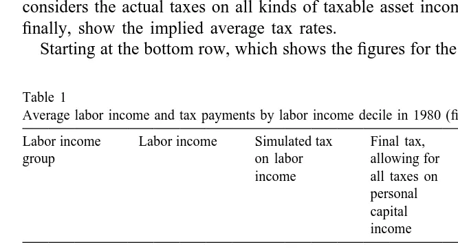
Edin (1990), and Edin et al. (1995). Also, the revenue statistics indicate that people claimed deductions to the extent that the personal capital income tax caused a substantial aggregate revenue loss. Further evidence is given in Table 1, where we reproduce the results of Malmer and Persson (1994), based on the 1980 cross-section of the income distribution survey of Statistics Sweden. Individuals are sorted into deciles by reported labor income. Column 1 reports the average labor income in each decile. Column 2 shows the tax (‘simulated tax’) that should have materialized if people’s only source of taxable income had been the labor income reported in the first column (allowing for the 1980 tax brackets, basic deductions, etc.). Column 3 shows the tax (‘final tax’) that materializes when one considers the actual taxes on all kinds of taxable asset income. Columns 4 and 5, finally, show the implied average tax rates.
Starting at the bottom row, which shows the figures for the average individual in
Table 1
a Average labor income and tax payments by labor income decile in 1980 (figures are in 1980 kronor) Labor income Labor income Simulated tax Final tax, Tax in percent
group on labor allowing for of labor income
income all taxes on
Simulated Final personal
capital income
1 2936 362 561 12.1 18.8
2 22,725 5971 5937 25.8 25.6
3 36,104 10,378 10,052 28.2 27.4
4 46,827 14,643 14,015 30.7 29.3
5 56,335 18,389 17,596 31.9 30.6
6 62,554 21,100 20,038 33.0 31.3
7 68,744 24,540 22,906 34.5 32.2
8 74,901 28,213 25,656 36.3 33.0
9 85,518 35,531 31,265 39.8 35.0
10 130,579 71,599 57,361 52.6 42.1
Total 58,722 23,078 20,543 38.1 33.9
a
Source: Malmer and Persson (1994), and the 1980 income distribution survey of Statistics Sweden. 2
the sample, we see that the deductions for interest expenses, realized capital losses, and private pension savings exceeded reported asset income by a substantial amount. As a consequence, the final tax falls short of the simulated one, and the average tax on labor income is lowered from 38.1 to 33.9%. But these tax reductions are very unevenly distributed. While the discrepancy between simulated and final tax rates is modest in the lower deciles, it is huge in the upper ones. Through various capital transactions the average individual in decile 10 lowered the average tax on labor income from 52.6 to 42.1%. Even more strikingly, Malmer and Persson report that a third of the individuals in the highest decile managed to reduce the final tax on labor income by more than 25%, and that a tenth of them halved the same tax rate.
From figures such as these it is hard to avoid the conclusion that Myrdal was more right than wrong, and that the formal rate of tax progression very much exaggerated the effective one. This interpretation is given further support by a study of Hansson and Norrman (1986), which concludes that the 1982 Swedish income tax can be characterized as de facto proportional. The Swedish experience does not seem to be unique. In their study of income tax avoidance in Germany, Lang et al. (1997) conclude that various legal and semi-legal tax write-off opportunities led to a dramatic reduction of the effective marginal tax rates of high-income households. For a discussion of the less clear-cut evidence for the US, see Gordon and Slemrod (1988).
3. The simple model
3.1. Labor supply
As a point of reference, assume first that no tax arbitrage is possible. Consider an individual with wage rate w, labor supply ,, and a time endowment normalized at unity. Given some tax schedule T(w,), the individual solves the optimization problem
Max u(c, 12,)
,
s.t. c5w,2T(w,).
Assuming that the problem is well-behaved, this gives rise to a labor supply function of the form
,5,(t, w) (1)
]
Consider now the implications of introducing tax avoidance in the form of trade in a perfect capital market. More specifically, we consider an economy with two types of assets, tax-exempt and taxable claims. We assume that no other form of wealth exists, and that the claims are inside assets, that is, people can freely issue both types of claims. This last assumption is a strong simplification (relaxed in Section 4), but it serves the useful purpose of illuminating the essence of the problem.
Denote by r the risk-free interest rate on taxable claims, and by r the risk-free interest rate on tax-exempt claims. As no individual has any initial wealth, a positive holding of taxable claims must be balanced by a negative holding of tax-exempt claims of the same amount, and vice versa. As a matter of convention, we let X denote borrowing against taxable claims. In line with a conventional global income tax we assume that the interest expense rX is fully deductible when 3 calculating taxable income. Taxable income B is thus (w,2rX ), and the tax paid is T(w,2rX ). Throughout we will assume that the tax schedule is continuously
4 differentiable, that 0#T9(.)#1, and that the tax schedule is progressive in the sense that T0(.).0. An individual with a wage rate w solves the following optimization problem:
Eq. (4) is our arbitrage condition, saying that the after-tax interest rate on taxable claims must equal the interest rate on tax-exempt claims. Since all individuals face the same relative asset yieldr/r in a perfect capital market, Eq. (4) implies that all individuals will have the same marginal tax rate T9(w,2rX ). Tax arbitrage will therefore transform the previously non-linear statutory tax schedule into an effective linear schedule with slope 12r/r. Also, since the marginal tax rate is a monotone function of taxable income, everybody will report the same taxable income:
21
9
w,2rX5T (12r/r) ; B(r/r). (5)
3
If the individual invests in taxable claims,2rX will be a positive number. 4
This is intuitively reasonable. With unlimited tax arbitrage, high-income in-dividuals issue taxable claims and hold tax-exempt claims, while low-income individuals hold taxable claims and issue tax-exempt claims. This process continues until all taxable incomes, and hence all marginal tax rates, are equalized. From an efficiency point of view, we may also note that this implies that
u (c,12,) r 2
]]]]5w .]
r u (c,12,)
1
In the presence of tax arbitrage, individual marginal rates of substitution between consumption and leisure are strictly proportional to the marginal rate of trans-formation (i.e. the wage rate). Since r and r are unequal, the factor of proportionality is to be regarded as a tax wedge.
Combining (3), (4), (5), and the budget constraint in (2), gives us labor supply ,and asset demand X (or, rather, the demand for interest deductions rX ):
,5,(r/r, w), (6)
rX5R(r/r, w). (7)
Since all individuals will be located at the same point on the tax schedule, we do not enter the vectort] as a separate argument in (6) and (7). However, it will still affect the form of the , and R functions. In the no-arbitrage case, however, individuals will be located at different points on the tax schedule. This is the reason why we explicitly enter t] as a separate argument in (1).
Here, one might of course ask why the government would choose a non-linear tax schedule if arbitrage would automatically make the effective tax schedule linear. The answer is either that the non-linear statutory schedule might be the result of some public choice mechanism that is outside the present model; or that the government, having not (yet) read this paper, incorrectly believes that it can impose a non-linear schedule.
The relative asset yield is determined by invoking equilibrium in the asset 5
market. We assume that all agents have identical preferences and differ only with respect to the wage rate w which, assuming a linear production technology, is the individual’s marginal and average productivity. In a Miller (1977) equilibrium, with purely inside assets, if follows that
E
XdF(w)50⇒ rE
XdF(w);E
R(r/r, w)dF(w)50 (8) where F(w) is the cumulative distribution function of wages. This condition determines r/r and thereby the effective marginal tax rate in the linearized tax5
schedule. It follows readily that an individual’s labor supply in general equilib-rium,,*, depends not only on her own wage but also on various moments of the overall wage distribution. Asset trade tends to link the labor supply decision to the wage structure, much in the same way as considerations of envy and interdepen-dent utility can produce demand and supply functions that depend on measures of
6 relative income.
We can obtain some characterizations of the equilibrium. Integrating (5) over all
]]
individuals, and using the Miller equilibrium condition (8), yields B(r/r)5w,*,
]]
where w,* is the average labor income in the economy. Substituting this back into (5), we obtain the individual’s demand for tax deductions in general equilibrium:
]]
rX*5w,*2w,*. (9)
As we should expect, individuals with a higher-than-average labor income have a positive demand for tax deductions, while the opposite holds for those with lower-than-average income. Individuals with average labor income will not participate in the arbitrage process. Also, when the tax system is purely redistributive, and when the government’s budget is balanced, there is a simple relation between the curvature of the tax schedule and the relative asset yield. An often adopted measure of the degree of tax progression is the measure of residual tax progression:
Our assumptions about the tax system imply that 0,v(B ),1. In equilibrium
]]
everyone has the same taxable income B5w,*. With a redistributive tax system
]] ]]
In equilibrium the relative asset yield equals the degree of tax progression of the formal bracket schedule, evaluated at the average labor income.
A logarithmic example. So far our analysis is quite general. It turns out,
however, that we can obtain surprisingly simple closed-form solutions for a particular parameterization of the model, namely a logarithmic utility function of the form
u(c, 12,)5ln c1aln (12,).
We also assume that the tax system is characterized by constant residual
6
progression in the sense that v in (10) is a constant. As shown by Jakobsson (1976), this means that disposable income out of a taxable income B is an exponential function of B:
v
B2T(B )5bB . (11)
Here, 0,v,1, and a lower value ofvmeans a higher degree of progressivity, in the sense of disposable income being a more concave function of taxable income. For a given v, we use the parameter b to ensure a balanced budget, and for simplicity, we only deal with a purely redistributive tax system. Within our arbitrage model, where everybody has the same taxable income, this implies
12v
T(B )50⇔b 5B . (12)
In an economy without arbitrage we get the labor supply function
v
]]
,5 . (13)
v1a
This corresponds to the supply function of the standard model (1), and it exhibits the well-known property that with logarithmic preferences and no initial wealth, labor supply is independent of the wage rate w.
In the arbitrage-economy, individual labor supply becomes
1 / (v21 )
1 a 12v r 1
]] ] ]]
S
D
] ],5
F
12S
?D G
(14)11a w v r bv
in partial equilibrium. We see that in an arbitrage-economy, modeling labor supply as (13) gives an incorrect functional form for the labor supply function. Using the general equilibrium condition (8), we can also solve for endogenous taxable income B(r/r): Substituting this into the partial equilibrium supply function (14), and using (12), gives us labor supply ,* in general equilibrium:
]
1 12v w
]]
S
]] ]D
,*5 12a ? . (15)
11a v1a w
Now, labor supply does depend on the wage rate even with logarithmic preferences and no other wealth. Comparing labor supply in the arbitrage and no-arbitrage economies, it follows that tax arbitrage leads to lower labor supply for
¯
3.2. Efficiency and tax incidence
The introduction of tax arbitrage could be the result of a conscious policy decision by the government, like deregulating the capital market, or making certain transactions legal that were not permitted under the earlier legislation. Or it could be the result of technological developments in financial markets that make asset trade possible at low transaction costs. In either case, it is interesting to know who would gain and who would lose from the introduction of tax arbitrage.
Let us first consider a regime where no tax arbitrage is possible. The indirect utility of an individual with a wage rate w, i.e. the utility resulting from labor supply (1) and its corresponding consumption, is denoted by V(w). Similarly, the indirect utility of the same individual under a regime where tax arbitrage is possible (i.e. the utility resulting from labor supply ,* and its corresponding consumption) is denoted by V (w), where the subscript stands for ‘arbitrage’. TheA
change in utility from introducing arbitrage is thus D;V (w)A 2V(w).
Assume now that the tax schedule is the same for the two cases (this assumption will be relaxed shortly). Then the introduction of tax arbitrage can make nobody worse off, since everybody can abstain from engaging in asset trade and supply exactly the same amount of labor as before. If someone nevertheless would choose to engage in asset trade, it would be only because this would yield higher utility. The change in relative price between consumption and leisure, from w(12
T9(w,)) to wr/r, would be greatest for people at the tails of the wage distribution. Thus these people would have the strongest incentives to trade with each other, high-income earners issuing taxable claims and purchasing tax-exempt ones, and
]
low-income earners doing the converse. People with average income w, would have nobody to trade with, and no incentive to do so. Thus they would supply the same amount of labor as before, and set X50.
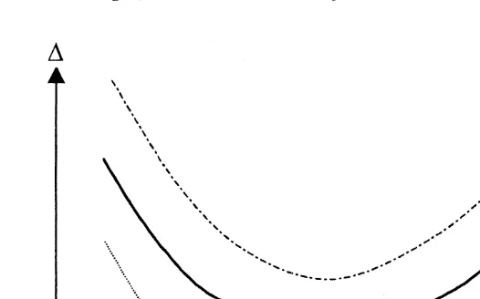
The utility gain from introducing tax arbitrage would therefore be greatest at the 7
tails of the wage distribution, and zero at the mean, as is illustrated by the middle curve in Fig. 1. Note, however, that this reasoning is based on the assumption of
8
an unchanged tax schedule. This is obviously unrealistic. Since the very purpose of tax arbitrage is to reduce taxes, it is reasonable to assume that the introduction of arbitrage would lead to a government budget deficit. In order to maintain budget balance, the government would thus have to raise taxes. Thus the average individual would not be unharmed by the introduction of tax arbitrage. Even if she does not engage in asset trade, she would be harmed by the tax increase and thus suffer a fall in utility. The distribution of Dover income groups would therefore
7
Other papers suggesting that tax arbitrage might benefit individuals at the tails of the income distribution include Gordon and Slemrod (1988), and Agell and Persson (1990).
8
Fig. 1. Distribution of utility gains from introducing tax arbitrage.
look like the lower curve in Fig. 1, showing a utility loss in the middle of the income distribution.
On the other hand, we cannot rule out that the introduction of tax arbitrage leads to a budget surplus rather than a deficit. This happens if the reduction of marginal tax rates for people with high wage rates leads to such a large increase in their labor supply that it outweighs the fall in labor supply among those with low wage rates. Then the tax base would increase, and the government could reduce taxes. Thus the average individual would gain from the introduction of tax arbitrage, as would everybody else. The distribution of utility gains would then look like the upper curve in Fig. 1.
How likely are these different cases? This is of course an empirical question. For the particular parameterization employed above (logarithmic preferences, iso-elastic tax schedule), the introduction of tax arbitrage will always necessitate a tax increase. Thus, people in the middle of the wage distribution will always lose. This presumes, however, that an average worker exists. What happens if this is not the case? Clearly, removal of people who do not exploit the scope for tax arbitrage, but pay additional taxes, increases the probability that there will be only
9 winners from the introduction of tax arbitrage.
Finally, two words of caution are warranted. Firstly, the reason why tax arbitrage might be a good thing, producing net gains for everyone, is simply that the initial non-linear tax schedule is arbitrarily chosen (possibly as the result of
9
some public-choice mechanism outside the model). It is therefore hardly surprising that an equally arbitrary linear tax schedule might result in a Pareto improvement. Secondly, in practice there are often real resource costs associated with many tax avoidance schemes, ranging from transactions costs and legal fees to costs associated with an inefficient allocation of risk, consumption, and productive capital. For example, since much tax avoidance activities involve real estate, an important cost probably consists of an oversized housing sector. Once we allow for such secondary excess burdens, the possibility that the introduction of tax arbitrage leads to a Pareto improvement gets smaller.
4. Introducing limitations to the arbitrage process
In the preceding section, we have seen how a simple arbitrage technology leads to labor supply responses that are quite different from the ones commonly analyzed in the literature. The most striking implication is that unlimited arbitrage leads to complete equalization of taxable incomes, and of the effective marginal tax rates on labor income. Although data for some countries indicate that tax avoidance leads to a substantial compression of the distribution of taxable income relative to the distribution of labor income, incomes are of course not completely equalized — a fact that suggests that there are limits to the arbitrage process. Obvious explanations are that imperfections in the capital market make it difficult to completely avoid taxation, or that the government is efficient in closing the
10
loopholes that open up for arbitrage. In this section we will explore two ways of incorporating such considerations in the analysis, limitations on short sales, and tax arbitrage in an asset that yields a direct utility service. We discuss the implications for applied work on labor supply and income distribution in Section 5.
4.1. Outside assets and constraints on short sales
As in the previous section, we model a situation when the only reason for asset trade is the desire to avoid taxation when marginal tax rates differ across individuals. But we now assume that the tax exempt asset is an outside asset in fixed supply, and that this asset (for simplicity referred to as land) cannot be sold short. We assume that land is productive, in the sense that each land unit produces
11
r units of the consumption good. The introduction of land means that there is an additional layer of heterogeneity. Each individual is now identified by a vector (w,
¯ ¯
X ), where X is the initial land endowment.
10
For a general discussion of how capital market imperfections and government regulations affect the scope for tax arbitrage, see Stiglitz (1983, 1985).
11
Asset trade proceeds as follows. At the beginning of the period, individuals exchange land endowments for taxable consumption loans. This exchange takes place at the per unit land price P. For any individual the proceeds from sales /
¯
purchases of land can then be written as P(X2X ), where X is the holding of land
at the end of the period, when production occurs. Due to the restriction on short sales, X$0. As there can be no net savings in our static model, any change in an individual’s land value is matched by a transaction of the opposite sign in the
¯
taxable asset. Specifically, an individual who spends a positive amount P(X2X )
on land increases tax deductible debt by the same amount. As before, r is the interest rate on the taxable asset.
The individual maximizes
where r;rP. The first-order conditions become
u (c, 12,) ]
The complementary slackness condition (18) has important implications for the shape of the labor supply function. Individuals who face a binding quantity constraint in the credit market react to different labor supply incentives than individuals who are at an interior portfolio optimum. Consider first the case of an interior solution, when (18) holds as an equality. For individuals with X.0, tax arbitrage is driven to the point where the after-tax return on the taxable asset equalsr. For these workers, the constraint on short sales is not an issue, and labor supply is determined in a way that parallels our previous analysis. The relevant
˜
marginal tax rate is the yield ratior/r, the same for everyone. It is easy to show that the behavioral functions take the form
¯
i.e. the tax system is linearized. Compared with the analysis in Section 3, the only novelty is that (19) and (20) include a wealth effect from the initial land endowment.
To derive the labor supply function for workers who are at a corner solution, we simply set X50 in (17). We then have
¯ ˜
,5,(t, w, rX ). (21)
For this group the labor supply function is quite similar to the one that materializes from the standard labor supply model in the presence of a nonlinear tax system,
¯ ˜
and an exogenous income from wealth, rX. In particular, the labor supply function includes a vector of parameters, t], describing global properties of the tax system. Although individuals at corners engage in intra-marginal asset trade, what matters for the form of the labor supply function is the extent of tax arbitrage on the margin.
To characterize the determination of equilibrium asset prices we need to derive the selection criterion that allocates individuals between the arbitrage and no-arbitrage regimes. Consider an individual for whom the non-negativity constraint is binding. For this individual we can write (18) as
r space that separates those who are at an interior optimum from those who are at a corner solution. For the particular case of a logarithmic utility function and a tax system with constant residual tax progression, analyzed in the previous section, the separating surface can be given a nice intuitive interpretation. After straight-forward but tedious manipulations, one can show that the separating hyperplane can be written as
Everybody with a full income w1rX less than the right-hand side of (22) will be
in a constrained optimum, while everybody with a full income that is greater than or equal to the right-hand side will be in an unconstrained optimum. Inherently poor individuals will face a binding credit constraint and a nonlinear tax system, and they will supply labor according to (21). Inherently rich individuals will face a perfect capital market and a linearized tax system, and they will supply labor according to (19).
We can now integrate (20) over all unconstrained individuals to obtain aggregate land demand. In equilibrium, this has to be equal to the total quantity of land available (which we for simplicity set equal to unity):
¯ ¯
˜ ˜ ˜
E
X(r/r, w, rX )dF(w, X )5r?1, (23)f(.)$0 ¯
where F(w, X ) now is a joint cumulative distribution function. Eq. (23) gives a
˜ ˜
solution for the endogenous variable r, or rather for the price of land, since r;rP.
incomes and effective marginal tax rates will now be the same only for that segment of the population which is at an interior portfolio optimum — an affluent subgroup consisting of those with high wages and / or large land endowments. Less affluent individuals do not hold the tax-exempt asset, and their taxable incomes vary across individuals.
Another observation is that constraints on short sales make it less likely that the introduction of tax arbitrage (via a policy decision, or as the consequence of technological innovation in financial markets) produces utility gains at both tails of the wage distribution. Although high-wage and low-wage individuals have strong incentives to engage in asset trade, the quantity constraint prevents low-wage individuals from going short in the tax-exempt asset. Thus, only high-wage individuals can reap the full reward from tax arbitrage. Finally, and very much in line with the analysis of the preceding section, we cannot rule out the possibility that tax arbitrage leads to such a boost to the labor supply of high-wage individuals, that the government can lower taxes. When the income tax distorts the labor supply decision of high-ability individuals to a great extent, everyone may benefit from the introduction of arbitrage.
4.2. When the tax-exempt asset is an argument in the utility function
In this subsection we briefly discuss a permutation, which turns out to have an interesting connection to the simple model of Section 3. Assume that the outside asset X appears as an argument in the utility function. Formally, this means a slight reformulation of (16), with X as an argument in the utility function, and with
r 50:
Max u(c, 12,, X )
,, X
(24)
] ]
˜ ˜
s.t. c5w,2r(X2X )2T(w,2r(X2X ))
where X is now an ordinary consumption good. In practice, we may think of X as housing, or some consumer durable. This model gives a representation of how housing, or durables, appear in the labor supply decision of an individual in an economy with full interest deductibility. Model (16) above has a closer re-semblance to a world where X is raw land (which gives a constant yield of the consumption good, but which does not appear in the utility function). Working out
¯ ˜
the first-order conditions gives us solutions for the supply of labor, ,(t, w, r, X ),
]
¯ ˜
and for the demand for housing, X(t], w, r, X ). These solutions will differ from those in Section 3 in the sense that both first-order conditions of (24) will involve marginal utilities. Several implications follow.
expenses had not been tax deductible. Thus the distribution of taxable income will be compressed relative to the wage distribution.
Secondly, consider an econometrician who ignores the fact that there are two consumption goods (c and X ), and incorrectly specifies the model as
Max u(c, 12,)
,
] ]
˜ ˜
s.t. c5w,2r(X2X )2T(w,2r(X2X )),
]
˜
where r(X2X ) is regarded as exogenously given non-labor income. Clearly, the
]
˜
implied labor supply function ,(t, w, r(X2X )) will be mis-specified, too. The
]
problems associated with this are not really due to the econometrician’s neglect of tax arbitrage per se, but rather to neglecting the fact that there are two consumption goods instead of one. The implications for the econometrics of labor supply of introducing a tax deductible good in the utility function is discussed by Triest (1992).
Finally, we have assumed that everyone consumes the same type of housing. In reality, people also make a tenure choice decision: low-income earners tend to consume rental housing, while high-income earners tend to live in their own houses. This suggests an arbitrage mechanism reminiscent of the simple model of Section 3. In that model, low-income earners issue tax-exempt claims and hold taxable ones, while high-income earners hold tax-exempt claims and issue taxable ones. In a housing market with tenure choice, a typical low-income earner pays a non-deductible rent to a landlord and has some taxable savings in the bank. The typical landlord is a high-income earner who has borrowed (tax-deductible) money from the bank in order to buy an apartment house, the income of which is in general favorably taxed. The payment streams are thus very similar: in both cases, low-income earners pay non-deductible and non-taxable (or lightly taxed) money to high-income earners, while high-income earners pay tax-deductible and taxable money to low-income earners.
5. Implications for empirical research
5.1. Econometrics of labor supply
In one form or another, the static labor supply function (1) — extended to include a measure of exogenous ‘non-labor income’ — has been at the center of attention in a large number of microeconometric studies that try to estimate how labor supply reacts to changes in economic incentives. Much of this literature has been preoccupied with the design of econometric techniques capable of dealing with nonlinear tax systems. In this process, the typical individual is modeled as maximizing utility with respect to work hours, subject to a nonlinear budget constraint that treats reported capital income as a given constant. This procedure creates three important problems.
Firstly, there is the issue of self-selectivity. As suggested by our model of constraints on short sales in Section 4.1, people will choose between two labor supply functions. For arbitrageurs (i.e. the inherently rich), labor supply is given by a functional form like (19). For individuals who face a binding constraint in the asset market (i.e. the inherently poor), some other functional form, like (21), applies. Econometric studies that build on the assumption that labor supply has the same functional form for everyone will come up with biased estimates.
Secondly, there is the issue of endogeneity of asset income. The standard procedure is to trace out individuals’ budget sets by changing the supply of hours, holding asset income constant. Under certain assumptions this will give a correct
local estimate of the marginal tax rate at the observed equilibrium point of the
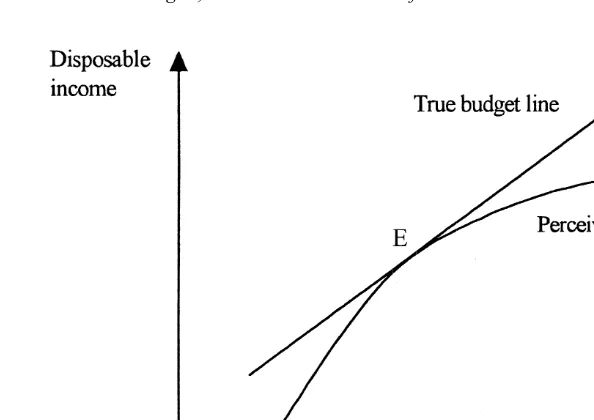
individual (provided that taxable and nontaxable asset incomes are correctly measured). Thus, even in the presence of tax arbitrage one may obtain a reliable estimate of how disposable income increases with an infinitesimal increase in individual labor supply. Since, however, asset income adjusts endogenously, the estimated marginal tax rate will exceed the effective marginal tax rate for any discrete change in labor supply. This is illustrated in Fig. 2. The concave curve shows consumption as a function of labor supply, given the statutory tax schedule, and holding asset income constant. The straight line shows the effective budget set, given that the individual engages in tax arbitrage. At the equilibrium point, E, the econometrician may derive a (local) estimate of the true marginal incentives
12
for labor supply. But the global incentives are shown by the straight line, rather than by the concave curve.
Thirdly, there is the issue of measurement error in asset income. The prime evidence about labor supply in Sweden, and in many other countries, stems from studies that rely on data from individuals’ tax returns. But the essence of tax arbitrage is that people invest their wealth in ways that are imperfectly measured or registered by the tax authorities. Our analysis suggests that the implied error in
12
Fig. 2. True and perceived budget constraints when asset income is measured without error.
the measurement of asset income will be correlated with the gross wage. The income tax returns of high-wage individuals will to a much greater extent than the income tax returns of low-wage individuals understate true asset income. Ceteris paribus, this systematic measurement error will tend to create a downward bias in the estimate of the gross wage coefficient. What the econometrician interprets as evidence of a backward bending labor supply function may simply reflect the influence of unobservable asset income.
Of course, the severity of these problems will differ quite a lot across countries, and between different time periods. In a situation with binding credit constraints, and low tax rates, it might be quite innocent to ignore the implications of tax arbitrage. Also, the problems may not be equally severe for all subgroups in the labor market. The econometric issues that we raise are likely to be of particular importance for the study of the labor supply decisions of the affluent. These individuals have much to gain from lowering their taxable income, and there is reason to believe that they have easier access to the credit market than other
13 people.
5.2. Income redistribution in the welfare state
A final observation is that our analysis casts strong doubt on the common use of tax return data in applied work on income distribution. According to several
13
studies Sweden ranks, together with some other high-tax countries, as one of the most egalitarian countries in the western industrialized world; see Gottschalk and Smeeding (1997). The Gini coefficient for reported disposable income is much smaller in Sweden than in the USA, a finding that is often attributed to the equalizing impact of progressive income taxes and transfers. But for reasons discussed in Section 5.1, the reliability of tax return data as an indicator of true economic income is likely to be a decreasing function of the tax rate. We would expect disposable income of the affluent, computed from the income tax returns, to underestimate actual disposable income. Because Swedish high-income earners are confronted with much higher tax rates than their US counterparts, this bias is likely to be larger in the Swedish than in the US data, thereby creating an impression of a much higher degree of equality in Sweden.
6. Concluding remarks
Our analysis rests on a number of strong assumptions. The analysis in Section 3 relies on the existence of a perfect asset market, and the analysis of capital market imperfections in Section 4 is specific rather than general. There are other ways of introducing assumptions that soften the stark prediction of equal taxable income, the most obvious one being perhaps to introduce uncertainty and risk aversion. This would make people less prone to engage in tax arbitrage to a full extent. Also, our models do not account for the fact that there is an intertemporal dimension to many tax arbitrage strategies (think of the postponed taxation associated with pension plans). Developing models that explore such alternative mechanisms seem like a worthwhile exercise.
We believe that research on how tax arbitrage interacts with labor supply decisions may shed light on a number of important questions concerning modern systems of income taxation. Firstly, what makes people work, given the very high marginal tax rates that can be observed for some countries during some periods? The traditional answer has been that labor supply is rather inelastic. Our proposed answer is different. With the tax avoidance technologies that became increasingly available during the 1980s, those who care about incentives need not pay those high tax rates.
Secondly, how come so many countries turned their tax systems into simple, 14
linear ones during the 1980s and 1990s? Our answer is that during this period, credit markets became increasingly well-functioning. Thus the effective tax schedules became more linear, and the reforms that were undertaken can be seen as a recognition of this fact.
Thirdly, the presence of tax arbitrage has potentially dramatic implications for the analysis of the optimal income tax along the lines of Mirrlees (1971). Tax
14
arbitrage implies that a large class of nonlinear optimal tax schedules will be hard to implement. Exploring models of optimal income taxation that are explicit about asset trade seems like an exciting research topic.
Fourthly, models that allow for tax arbitrage and asset trade have important implications for the econometric analysis of labor supply, and for applied work on income distribution. Studies that ignore the effect of tax arbitrage and asset trade on labor supply incentives will come up with biased estimates of important elasticities, and international comparisons of income inequality will exaggerate the redistributive achievements of high-tax countries like Sweden.
Fifthly, how does tax avoidance affect estimates of the deadweight burden of the income tax? Feldstein (1995) argues that models that account for tax avoidance will produce calculations of excess burdens that are many times larger than those implied by standard Harberger-calculations. A contrary view, from the perspective of a high-tax country, is that tax avoidance may be seen ‘ . . . as a means of blowing off some steam in order to save the engine from exploding’ (Lindencrona, 1993, p. 166). Our analysis shows that it is easy to develop models where asset trade reduces the efficiency cost of income taxation. In the end, whether tax avoidance leads to smaller or greater excess burdens is an empirical question, that depends on country-specifics, like the structure of the tax system, the type of available arbitrage technologies, etc.
Sixthly, from a public choice perspective tax arbitrage and a highly progressive tax system can be viewed as an ingenious way of reconciling incompatible political ambitions. High marginal tax rates convey the message that politicians care about the less well off, while a generous attitude towards tax avoidance prevents the very same tax system from destroying the incentives of the rich and the highly educated. The political economy of tax design seems like an important research topic for the future.
Acknowledgements
´
¨ ´
We thank Dan Anderberg, Axel Borsch-Supan, Roger Gordon, Angel Lopez ´
Nicolas, Søren Bo Nielsen, Shlomo Yitzhaki, and two referees for comments. We have benefited from presentations at the 1998 Trans-Atlantic Public Economics Seminar, Swedish Ministry of Finance, and the Universities of Aarhus, Bergen,
˚
and Umea. We thank Annika Persson of the National Tax Board for providing us with the data in Table 1.
References
¨
Agell, J., Englund, P., Sodersten, J., 1998. Incentives and Redistribution in the Welfare State — the Swedish Tax Reform. Macmillan Press, Basingstoke.
Agell, J., Persson, M., 1990. Tax arbitrage and the redistributive properties of progressive income taxation. Economics Letters 34, 357–361.
Agell, J., Persson, M., 1998. Tax arbitrage and labor supply. NBER, Working paper 6708; August. Allingham, M.G., Sandmo, A., 1972. Income tax evasion: a theoretical analysis. Journal of Public
Economics 1, 323–338.
Auerbach, A., Slemrod, J., 1997. The economic effects of the tax reform act of 1986. Journal of Economic Literature 35, 589–632.
Blomquist, S., 1996. Estimation methods for male labor supply functions. How to take account of nonlinear taxes. Journal of Econometrics 70, 383–405.
Cowell, F.A., 1990. Cheating the Government: the Economics of Evasion. The MIT Press, Cambridge, MA.
˚
Edin, P.-A., Englund, P., Ekman, E., 1995. Avregleringen och hushallens skulder (Deregulation and household indebtedness). In: Bankerna under krisen (The banks during the crisis).
Bankkriskom-´
mitten, Stockholm.
Feldstein, M., 1995. Tax avoidance and the deadweight loss of the income tax. NBER, Working paper no. 5055; March.
Gordon, R., Slemrod, J., 1988. Do we collect any revenue from taxing capital income. In: Summers, L. (Ed.), Tax Policy and The Economy. MIT Press, Cambridge, MA.
Gottschalk, P., Smeeding, T., 1997. Cross-national comparisons of earnings and income inequality. Journal of Economic Literature 35, 633–687.
¨
Hansson, I., Norrman, E., 1986. Fordelningseffekter av inkomstskatt och utgiftsskatt (Distributional effects of income taxation and expenditure taxation). In: SOU, Vol. 40, 1986, Stockholm. Hausman, J., 1981. Labor supply. In: Aaron, H.J., Pechman, J.A. (Eds.), How Taxes Affect Economic
Behavior. Brookings Institution, Washington DC.
Jakobsson, U., 1976. On the measurement of the degree of progression. Journal of Public Economics 5, 161–168.
¨
Lang, O., Nohrbaß, K.-H., Stahl, K., 1997. On income tax avoidance: the case of Germany. Journal of Public Economics 66, 327–347.
Lindbeck, A., 1995. Hazardous welfare-state dynamics. American Economic Review (Papers and Proceedings) 85, 9–15.
Lindencrona, G., 1993. The taxation of financial capital and the prevention of tax avoidance. In: Tax reform in the Nordic countries, 1973–1993. Jubilee Publication. The Nordic Council for Tax Research, Iustus, Uppsala.
MaCurdy, T.E., Green, D., Paarsch, H., 1990. Assessing empirical approaches for analyzing taxes and labor supply. Journal of Human Resources 25, 415–490.
˚
Malmer, H., Persson, A., 1994. Skattereformens effekter pa skattesystemets driftskostnader, skatteplan-ering och skattefusk (The effects of the tax reform on compliance costs, tax planning, and tax
˚ ˚
fraud). In: Malmer, H., Persson, A., Tengblad, A (Eds.), Arhundradets skattereform (Tax reform of the century). Fritzes, Stockholm.
Mayshar, J., 1991. Taxation with costly administration. Scandinavian Journal of Economics 93, 75–88. Miller, M., 1977. Debt and taxes. Journal of Finance 32, 261–275.
Mirrlees, J., 1971. An exploration in the theory of optimum income taxation. Review of Economic Studies 38, 175–208.
Moffitt, R., Wilhelm, M., 1998. Taxation and the labor supply decisions of the affluent. Johns Hopkins University, Mimeo.
¨
Myrdal, G., 1978. Dags for ett nytt skattesystem (Time for a new tax system). Ekonomisk Debatt 6, 493–506.
Persson, M., 1995. Why are taxes so high in egalitarian societies? Scandinavian Journal of Economics 97, 569–580.
Sandmo, A., 1981. Income tax evasion, labour supply, and the equity-efficiency tradeoff. Journal of Public Economics 16, 265–288.
Sandmo, A., 1991. Economists and the welfare state. European Economic Review 35, 213–239. Slemrod, J., 1994. A general model of the behavioral response to taxation. University of Michigan,
Mimeo.
Sørensen, P.B., 1994. From the global income tax to the dual income tax: recent tax reforms in the Nordic countries. International Tax and Public Finance 1, 57–79.
Stiglitz, J., 1983. Some aspects of the taxation of capital gains. Journal of Public Economics 21, 257–294.
Stiglitz, J., 1985. The general theory of tax avoidance. National Tax Journal 38, 325–337.
Summers, L., Gruber, J., Vergara, R., 1993. Taxation and the structure of labor markets: the case of corporatism. Quarterly Journal of Economics 108, 385–411.