El e c t ro n ic
Jo ur
n a l o
f P
r o
b a b il i t y
Vol. 16 (2011), Paper no. 6, pages 174–215. Journal URL
http://www.math.washington.edu/~ejpecp/
A central limit theorem for random walk in a random
environment on marked Galton-Watson trees
Gabriel Faraud
∗Abstract
Models of random walks in a random environment were introduced at first by Chernoff in 1967 in order to study biological mechanisms. The original model has been intensively studied since then and is now well understood. In parallel, similar models of random processes in a random environment have been studied. In this article we focus on a model of random walk on random marked trees, following a model introduced by R. Lyons and R. Pemantle (1992). Our point of view is a bit different yet, as we consider a very general way of constructing random trees with random transition probabilities on them. We prove an analogue of R. Lyons and R. Pemantle’s recurrence criterion in this setting, and we study precisely the asymptotic behavior, under re-strictive assumptions. Our last result is a generalization of a result of Y. Peres and O. Zeitouni (2006) concerning biased random walks on Galton-Watson trees.
Key words: Random Walk, random environment, tree, branching random walk, central limit theorem.
AMS 2000 Subject Classification:Primary 60K37; 60F05; 60J80.
Submitted to EJP on July 13, 2010, final version accepted December 22, 2010.
∗Laboratoire Analyse, Géométrie et Applications, UMR 7539, Institut Galilée, Université Paris 13, 99 avenue J.B.
1
Introduction and statement of results.
Models of random walks in a random environment were introduced at first by Chernov in 1967 ([6]) in order to study biological mechanisms. The original model has been intensively studied since then and is now well understood. On the other hand, more recently, several attempts have been made to study extensions of this original model, for example in higher dimensions, continuous time, or different space.
It is remarkable that the random walk inZd,d>1, is still quite mysterious, in particular no precise criterion for recurrence/transience has ever been found.
In the case of trees, however, a recurrence criterion exists, and even estimates for the asymptotic behavior have been proven. To present our model and the existing results, we begin with some notations concerning trees. LetT be a tree rooted at some vertexe. For each vertex x ofT we call
N(x)the number of his children{x1,x2, ...,xN(x)}, and←x−his father. For two vertices x,y ∈T, we calld(x,y)the distance between x and y, that is the number of edges on the shortest path from x
to y, and |x|:= d(e,x). LetTn be the set of vertices such that|x|= n, and T∗ =T\ {e}. We also note x< y whenx is an ancestor of y.
We call a marked tree a couple(T,A), whereAis a random application from the vertices ofT toR∗
+.
LetTbe the set of marked trees. We introduce the filtrationGnonTdefined as
Gn=σ{N(x),A(xi), 1≤i≤n,|x|<n,x ∈T}.
Following[20], given a probability measureqonN⊗R∗N∗
+ , there exists a probability measureMTon
Tsuch that
• the distribution of the random variable(N(e),A(e1),A(e2), ...)isq,
• givenGn, the random variables(N(x),A(x1),A(x2), ...), forx ∈Tn, are independent and their conditional distribution isq.
We will always assumem:=E[N(e)]>1, ensuring that the tree is infinite with a positive probability.
We now introduce the model of random walk in a random environment. Given a marked treeT, we set for x∈T∗,xi a child ofx,
ω(x,xi) =
A(xi)
1+PNj=(1x)A(xj)
and
ω(x←−x ) = 1 1+PNj=(1x)A(xj)
.
Morever we setω(x,y) =0 wheneverd(x,y)6=1,
It is easy to check that(ω(x,y))x,y∈T is a family of non-negative random variables such that,
∀x ∈T,X y∈T
ω(x,y) =1,
and
∀x ∈T∗,A(x) = ω(
←x−,x)
ω(←−x,←←x−−)
whereω(e,←−e)is artificially defined as
1
ω(e,←−e) =
X
|x|=1
A(x).
Further,ω(x,y)6=0 wheneverx and y are neighbors.
T will be called “the environment”, and we call “random walk on T” the Markov chain (Xn,PT) defined byX0=eand
∀x,y ∈T, PT(Xn+1= y|Xn= x) =ω(x,y). We call “annealed probability” the probabilityP
MT=MT⊗PT taking into account the total alea. We set, forx∈T,Cx=Qe<z≤xA(z). We can associate to the random walkXnan electrical network with conductance Cx along[←x−,x], and a capacited network with capacity Cx along [←x−,x]. We recall the definition of an electrical current on an electrical network. LetG = (V,E)be a graph, C
be a symmetric function onE, andA,Zbe two disjoint subsets ofV. We define the electrical current betweenAandZas a functionithat is antisymmetric onEsuch that, for anyx ∈V\(A∪Z), the sum on the edgesestarting from x ofi(e)equals zero (this is call Kirchhoff’s node Law), and, moreover,
isatisfies the Kirchhoff’s cycle Law, that is, for any cycle x1,x2, . . . ,xn=x1,
n
X
i=1
i(xi,xi+1)
C(xi,xi+1)=0.
A flow on a capacited network is an antisymmetric functionθthat satisfies the Kirchhoff’s node Law, and such that, for all edgese,θ(e)<C(e), (for more precisions on this correspondence we refer to the chapters 2 and 3 of[17]).
We shall also frequently use the convex functionρdefined forα≥0 as
ρ(α) =EMT
N
(e)
X
0
A(ei)α
=Eq
XN
0
A(i)α
.
Remark : This model is in fact inspired by a model introduced in[16]. In this case the tree T and theA(x)were introduced separately, and theA(x)were supposed to be independent. Here we can include models in which the structure of the tree and the transition probabilities are dependent. A simple example that is covered in our model is the following : Let T be a Galton-Watson tree. We chose an i.i.d. family (B(x))x∈T and set, for every x ∈T, 1≤ i≤ N(x), A(xi) = B(x). This way the transition probabilities to the children of any vertex are all equal, but randomly chosen. In R. Lyons and R. Pemantle’s article, a recurrence criterion was shown, our first result is a version of this criterion in our setting.
Theorem 1.1. We suppose that there exists0≤ α≤1such that ρis finite in a small neighborhood of α, ρ(α) =inf0≤t≤1ρ(t):= p and ρ′(α) = Eq
hPN(e)
i=1 A(ei)αlog(A(ei))
i
is finite. We assume that
PN(e)
i=1 A(ei)is not identically equal to1.
Then,
1. if p<1then the RWRE is a.s. positive recurrent, the electrical network has zero conductance a.s.,
2. if p≤1then the RWRE is a.s. recurrent, the electrical network has zero conductance a.s. and the capacited network admits no flow a.s..
3. if p>1, then, given non-extinction, the RWRE is a.s. transient, the electrical network has positive
conductance a.s. and the capacited network admits flow a.s..
(By “almost surely” we mean “forMTalmost every T ”).
Remark: In the case wherePNi=(1e)A(ei)is identically equal to 1, which belongs to the second case,
|Xn| is a standard unbiased random walk, therefore Xn is null recurrent. However, there exists a flow, given byθ(←−x,x) =Cx.
The proof of this result is quite similar to the proof of R. Lyons and R. Pemantle, but there are some differences, coming from the fact that in their settingi.i.d. random variables appear along any ray of the tree, whereas it is not the case here. Results on branching processes will help us address this problem.
Theorem 1.1 does not give a full answer in the casep=1, but this result can be improved, provided some technical assumptions are fulfilled. We introduce the condition
(H1): ∀α∈[0, 1], Eq
N
(e)
X
0
A(ei)α
log+
N
(e)
X
0
A(ei)α
<∞,
In the critical case, we have the following
Proposition 1.1. We suppose p = 1, m > 1 and (H1). We also suppose that ρ′(1) =
EqhPNi=(1e)A(ei)log(A(ei))iis defined and thatρis finite in a small neighborhood of1. Then,
• ifρ′(1)<0, then the walk is a.s. null recurrent, conditionally on the system’s survival,
• ifρ′(1) =0and for someδ >0,
EMT[N(e)1+δ]<∞,
then the walk is a.s. null recurrent, conditionally on the system’s survival,
• ifρ′(1)>0,and if for someη >0,ω(x,←−x )> ηalmost surely, then the walk is almost surely
positive recurrent.
Remark: The distinction between the caseρ′(1) =0 andρ′(1)>0 is quite unexpected.
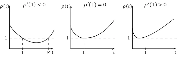
The study of the critical case turns out to be quite interesting, indeed several different behaviors appear in this case. The quantityκ=inf{t>1,ρ(t)>1}, associated toqis of particular interest. Whenρ′(1)≥0, for regular trees and identically distributed A(x), Y. Hu and Z. Shi showed ([9]) that there exist constants 0<c1≤c2<∞such that
c1≤lim infn →∞
max0<s<n|Xs|
(logn)3 ≤lim sup
n→∞
max0<s<n|Xs|
(logn)3 ≤c2, P−a.s..
It was recently proven by G. Faraud, Y. Hu and Z. Shi that max0<s<n|Xs|
(logn)3 actually converges to an
1 1 1
ρ(t) ρ(t) ρ(t)
t t t
ρ′(1)<0 ρ′(1) =0 ρ′(1)>0
1 κ 1 1
Figure 1: Possible shapes forρin the critical case
In the caseρ′(1)<0, Y. Hu and Z. Shi showed ([8]) that
lim n→∞
log max0<s<n|Xs| logn =1−
1
min{κ, 2}, P−a.s..
Results in the casep<1 have also been obtained by Y. Hu and Z. Shi ([8]), and the casep>1 has been studied by E. Aidekon ([1]).
Let us go back to the critical case. Our aim is to study what happens whenκis large. Whenκ≥2, the walk behaves asymptotically like n12. Our aim is to get a more precise estimate in this case.
However we are not able to cover the whole regimeκ∈[2,∞].
We first introduce the ellipticity assumptions
∃0< ǫ0<∞;∀i,ǫ0≤A(ei)≤ 1
ǫ0
,q−a.s. (2)
and we assume that(A(ei))1≤i≤N(e)is of the form(A′(i)1(i≤N(e))i≥1, where(A′(i))i≥1is a i.i.d. family independent ofN(e)and that Eq[N(e)κ+1]<∞. (H2)
Remark :We actually only need this assumption to show Lemma 4.3, we can, for example, alterna-tively suppose that
∃N0;N(e)≤N0,q−p.s. etPq[N≥2|A(e1)]≥ 1
N0
(3)
Note furthermore that those conditions imply (H1).
Theorem 1.2. Suppose N(e)≥1, q−a.s., (2), (3).
If p = 1, ρ′(1) <0 and κ∈(8,∞], then there is a deterministic constant σ >0 such that, forMT
almost every tree T, the process{|X⌊nt⌋|/
p
σ2n}converges in law to the absolute value of a standard
Brownian motion, as n goes to infinity.
Remark :This result is a generalization of a central limit theorem proved by Y. Peres and O. Zeitouni [21]in the case of a biased standard random walk on a Galton-Watson tree. In this case,A(x)is a constant equal to m1, thereforeκ=∞. Our proof follows the same lines as theirs.
In the annealed setting, things happen to be easier, and we can weaken the assumption onκ.
Theorem 1.3. Suppose N(e)≥1, q−a.s., (2), (3). If p=1,ρ′(1)<0andκ∈(5,∞], then there is
a deterministic constantσ >0such that, underPMT, the process{|X⌊nt⌋|/
p
σ2n}converges in law to
Remark : As we will see, the annealed CLT will even be true for κ ∈(2,∞), on a different kind of tree, following a distribution that can be described as “the invariant distribution” for the Markov chain of the “environment seen from the particle”.
We thank P. Mathieu for indicating to us the technique of C. Kipnis and S.R.S. Varadhan ([12]), that was quite an inspiration for us.
Our article will be organized as follows
• In section 2 we show Theorem 1.1.
• In section 3 we introduce a new law on trees, with particular properties.
• In section 4 we show a Central Limit Theorem for random walks on trees following the “new law”.
• In section 5 we expose a coupling between the original law and the new one.
• In section 6 we show some lemmas.
• In section 7 we show Theorem 1.3
2
Proof of Theorem 1.1.
Let us first introduce an associated martingale, which will be of frequent use in the sequence.
Letα∈R+and
Yn(α)= X
x∈Tn Y
e<z≤x
A(z)α= X
x∈Tn
Cαx.
Yn(α)is known as Mandelbrot’s Cascade.
It it is easy to see that ifρ(α)<∞then Y (α)
n
ρ(α)n is a non-negative martingale, with a.s. limitY
(α).
We have the following theorem, due to J.D. Biggins (1977) (see[3, 4]) that allows us to know when
Y(α)is non trivial.
Statement 2.1(Biggins). Letα∈R+. Supposeρ is finite in a small neighborhood ofα, and ρ′(α)
exists and is finite, then the following are equivalent
• given non-extinction, Y(α)>0a.s.,
• PMT[Y(α)=0]<1,
• EMT[Y(α)] =1,
• EqhP0N(e)A(ei)αlog+PN0(e)A(ei)αi<∞, and
(H2):=αρ′(α)/ρ(α)<logρ(α),
This martingale is related to some branching random walk, and has been intensively studied ([18, 3, 4, 13, 14, 19]). We will see that it is closely related to our problem.
Let us now prove Theorem 1.1. We shall use the following lemma, whose proof is similar to the proof presented in page 129 of[16]and omitted.
Lemma 2.1.
min
0≤t≤1E
X
x∈T1 A(x)t
= max
0<y≤1tinf>0y 1−tE
X
x∈T1 A(x)t
.
(1) Let us begin with the subcritical case, We suppose there exists some 0 < α < 1 such that
ρ(α) = inf0≤t<1ρ(t) < 1. Then, following [11] (Prop 9-131), and standard electrical/capacited
network theory, if the conductances have finite sum, then the random walk is positive recurrent, the electrical network has zero conductance a.s., and the capacited network admits no flow a.s.. We have
X
x∈T∗
Cxα= ∞ X
n=0 X
x∈Tn
Cαx =X
n
ρ(α)nYn(α).
SinceYn(α)is bounded (actually it converges to 0), we have
X
x∈T∗
Cαx <∞, MT−a.s..
This implies thata.s., for all but finitely many x,Cx <1, and thenCx ≤Cxα, which gives the result.
(2)As before, we haveα such that ρ(α) =inf0≤t≤1ρ(t)≤ 1. We have to distinguish two cases.
Eitherρ′(1)≥0, therefore it is easy to see that, forα, (H2) is not verified, so
X
x∈Tn
Cxα=Yn(α)→0,
when n goes to∞. Then fornlarge enough,Cx <1 for every x∈Tn, whence
X
x∈Tn
Cx→0,
then by themax-flow min-cut theorem, the associated capacited network admits no flow a.s., this implies that no electrical current flows, and that the random walk is recurrentMT-a.s..
We now deal with the case whereρ′(1)<0, thenα=1. The proof is similar to[16], but, as it is quite short, we give it for the sake of clarity. We use the fact that, if the capacited network admits no flow frome, then the walk is recurrent.
We call F the maximum flows fromein T, and for x∈T, |x|=1, we call Fx the maximum flow in the subtree Tx ={y ∈T,x ≤ y}, with capacity AC(xy) along the edge (←x−,x). It is easy to see that F
andFx have the same distribution, and that
F= X
|x|=1
Taking the expectation yields
E[F] =E[Fx∧1] =E[F∧1],
thereforeesssupF≤1. By independence, we obtain from (4) that
esssupF = (esssup X
|x|=1
A(x))(esssupF).
This implies thatF =0 almost surely, as(esssupP|x|=1A(x))>1, whenP|x|=1A(x)is not identi-cally equal to 1 .
(3)We shall use the fact that, if the water flows whenCx is reduced exponentially in|x|, then the electrical current flows, and the random walk is transient a.s. (see[15]).
We have
inf
α∈[0,1]E
N
(e)
X
0
A(ei)α
=p>1
(pcan be infinite, in which case the proof still applies).
We introduce the measureµn defined as
µn(A) =E[♯(A∩ {logCx}x∈Tn)],
where♯denotes the cardinality.
One can easily check that
φn(λ):=
Z +∞
−∞
eλtdµn(t) =E
X
x∈Tn
Cxλ
=ρ(λ)n.
Let y ∈(0, 1]be such that p =inft>0y1−tE[ P
x∈T1A(x)
t]. Then, using Cramer-Chernov theorem
(and the fact that the probability measureµn/mn has the same Laplace transform as the sum ofn independent random variables with lawµ1/m), we have
1
nlogµn([n(−logy),∞))→log(p/y).
Now, if we set 1/y<q<p/y, there exists ksuch that
E[♯{x ∈Tk|Cx > yk}]>qk.
Then the end of the proof is similar to the proof in[16]. We chose a smallε >0 such that,
E[♯{x ∈Tk|Cx > yk, and∀e<z≤x,A(z)> ε}]>qk.
Let Tk be the tree whose vertices are {x ∈Tkn,n∈N}such that x =←−y in Tk iff x ≤ y in T and
|y|=x+k. We form a random subgraphTk(ω)by deleting the edges(x,y)where
Y
x<z≤y
LetΓ0 be the connected component of the root. The treeΓ0 is a Galton-Watson tree, such that the expected number of children of a vertex isqk > 1, hence with a positive probabilityΓ0 is infinite and has branching number overqk.
Using Kolmogoroff’s 0-1 Law, conditionally to the survival there is almost surely a infinite connected component, not necessarily containing the root. This connected component has branching number at leastqk. Then we can construct almost surely a subtree T′ ofT, with branching number overq, such that∀x ∈T′,A(x)> εand if|x|=nk,|y|= (n+1)kandx < y thenQx<z≤yA(z)>qk. This implies the result.
We now turn to the proof of Proposition 1.1. Letπbe an invariant measure for the Markov chain (Xn,PT)(that is a measure onT such that,∀x∈T,π(x) =Py∈Tπ(y)ω(y,x)), then one can easily check that
π(x) = π(e)ω(e,
←−e)
ω(x,←x−)
Y
0<z≤x
A(z),
with the convention that a product over an empty set is equal to 1.
Then almost surely there exists a constantc>0 (dependant of the tree) such that
π(x)>c Cx.
Thus X
x∈T
π(x)>cX
n
Yn(1).
-Ifρ′(1)<0, then (H2) is verified andY >0 a.s. conditionally to the survival of the system, thus the invariant measure is infinite and the walk is null recurrent.
-Ifρ′(1) =0, we use a recent result from Y. Hu and Z. Shi. In[10] it was shown that, under the assumptions of Theorem 1.1, there exists a sequenceλn such that
0<lim inf n→∞
λn
n1/2 ≤lim supn→∞ λn
n1/2 <∞
andλnYn(1)→n→∞Y, withY >0 conditionally on the system’s survival. The result follows easily.
-If ρ′(1) > 0, there exists 0 < α < 1 such thatρ(α) = 1, ρ′(α) = 0. We set, for every x ∈ T, ˜
A(x):=A(x)α. We set accordingly ˜C(x) =Q0<z≤xA˜(z), and
˜
ρ(t):=Eq
N
(e)
X
i=1
˜
A(ei)t
=ρ(αt).
Note that ˜ρ(1) = 1 = inf0<t≤1ρ(t) and ˜ρ′(1) = 0. Note that under the ellipticity condition ω(x,←x−)> η, for some constantc>0
X
x∈T
π(x)<cX
x∈T
Cx =X
x∈T ˜
C1x/α.
Using Theorem 1.6 of[10]withβ=1/αand ˜Cx =e−V(x), we get that for any 23α <r< α,
EMT
X
x∈Tn
Cx
r
Note that asr<1,
X
n
Yn(1)
r
≤X
n
Yn(1)r,
whence, using Fatou’s Lemma,
EMT
X
x∈T
Cx
!r
<∞.
This finishes the proof.
3
The
IMT
law.
We consider trees with a marked ray, which are composed of a semi infinite ray, calledRa y={v0=
e,v1 =←v−0,v2=←v−1...}such that to eachvi is attached a tree. That wayvi has several children, one of which beingvi−1.
As we did for usual trees, we can “mark” these trees with{A(x)}x∈T. Let ˜Tbe the set of such trees. LetFn be the sigma algebraσ(Nx,Axi,vn ≤x) andF∞=σ(Fn,n≥0). While unspecified,
“mea-surable” will mean “F∞- measurable”.
Letqˆbe the law onN×R∗N∗
+ defined by
dˆq
dq =
NX(e)
1
A(ei).
Remark : For this definition to have any sense, it is fundamental that Eq[
PN(e)
1 Ai] =1, which is provided by the assumptionsρ′(1)<0 andp=1.
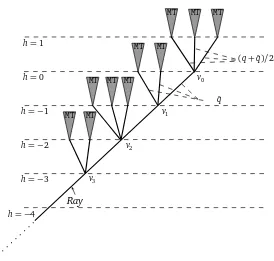
Following [21], let us introduce some laws on marked trees with a marked ray. Fix a vertex v0
(the root) and a semi infinite ray, calledRa y emanating from it. To each vertexv∈Ra ywe attach independently a set of marked vertices with lawqˆ, except to the rooteto which we attach a set of children with law(q+ ˆq)/2. We chose one of these vertices, with probability PA(vi)
A(vi), and identify it
with the child of v onRa y. Then we attach a tree with lawMTto the vertices not onRa y. We call
IMTthe law obtained.
We callθvT be the treeT “shifted” to v, that is,θvT has the same structure and labels as T, but its root is moved to vertexv.
Note that as before, given a treeT in ˜T, we can define in a unique way a familyω(x,y)such that
ω(x,y) =0 unlessd(x,y) =1,
∀x ∈T,X y∈T
ω(x,y) =1,
and
∀x∈T,A(x) = ω(
←x−,x)
ω(←x−,←←−−x )
. (5)
We call random walk on T the Markov chain(Xt,PT) on T, starting from v0 and with transition
MT MT
MT MT MT MT MT
MT MT MT
v0
v1
v2
v3
h=1
h=0
h=−1
h=−2
h=−3
h=−4
(q+ ˆq)/2
ˆ q
Ray
Figure 2: TheIMTlaw.
Let Tt = θXtT denote the walk seen from the particle. T
t is clearly a Markov chain on ˜T. We set, for any probability measureµon ˜T,Pµ=µ⊗PT the annealed law of the random walk in a random environment on trees following the lawµ. We have the following
Lemma 3.1. IMTis a stationnary and reversible measure for the Markov process Tt, in the sense that,
for every F : ˜T2→Rmeasurable,
EIMT[F(T0,T1)] =EIMT[F(T1,T0)].
Proof : Suppose G is aFn-measurable function, that is, G only depends on the (classical) marked tree of the descendants of vn, to which we will refer asT−nand on the position of v0 in then−th
level ofT−n. We shall write accordinglyG(T) =G(T−n,v0)
We first show the following
Lemma 3.2. If G isFn measurable, then
EIMT[G(T)] =EMT
X
x∈Tn
CxG(T,x)
1+PA(xi) 2
. (6)
Remark : These formulae seem to create a dependency on n, which is actually irrelevant, since
Eq[PiN=(1e)A(ei)] =1.
Proof : This can be seen by an induction overn, using the fact that
EIMT[G(T−n,v0)] =Eq
XN
i=1
A(ei)E
G(T′(i,N,A(ej)),v0)|i,N,A(ej)
where T′(x,N,A(ei))is a tree composed of a vertexvn withN children marked with theA(ei), and on each of this children is attached a tree with lawMT, except on the i-th, where we attach a tree whose law is the same asT−(n−1).
Iterating this argument we have
EIMT[G(T−n,v0)] =EMT
MTtrees. The result follows.
Let us go back to the proof of Lemma 3.1. Using the definition of the random walk, we get
E
It is easily verified that
∀x,y ∈T,ω(x,y)1+
Using this equality, we get
E
4
The Central Limit Theorem for the RWRE on
IMT
Trees.
In this section we introduce and show a central limit theorem for random walk on a tree following the law IMT. For T ∈ T˜, let h be the horocycle distance on T (see Figure 2). hcan be defined
recursively by (
h(v0) =0
h(←x−) =h(x)−1, ∀x ∈T.
We have the following
Theorem 4.1. Suppose p = 1, ρ′(1) < 0and κ∈[5,∞], as well as assumptions (2) and (H2) or
(3). There exists a deterministic constantσsuch that, forIMT−a.e.T,the process{h(X⌊nt⌋)/pσ2n}
converges in distribution to a standard Brownian motion, as n goes to infinity.
The proof of this result consists in the computation of a harmonic functionSx on T. We will show that the martingaleSX
t follows an invariance principle, and then thatSx stays very close toh(x).
Let, forv∈T,
Wv =lim
n
X
x∈T,v<x,d(v,x=n)
Y
v<z≤x
A(z).
Statement 2.1 implies thatWv >0a.s. andE[Wv|σ(A(xi),N(x),x < v)] =1. Now, let M0=0 and ifXt=v,
Mt+1−Mt=
¨
−Wv if Xt+1=←v−
Wv
i, ifXt+1=vi
.
GivenT, this is clearly a martingale with respect to the filtration associated to the walk. We intro-duce the functionSx defined asSe=0 and for allx ∈T,
Sxi =Sx+Wxi, (7)
in such a way thatMt=SXt.
Let
η=EGW[W02], (8)
which is finite due to Theorem 2.1 of[13](the assumption needed for this to be true isκ >2). We call
Vt:= 1
t
t
X
i=1
ET[(Mi+1−M i)2|Ft]
the normalized quadratic variation process associated toMt. We get
ET[(Mi+1−M i)2|Ft] =ω(Xi,←X−i)WX2i+
NX(Xi)
j=1
ω(Xi,Xi j)WX2i j=G(Ti),
whereXi j are the children ofXi andG is a L1(IMT)function on ˜T(again due toκ >2).
Let us defineσsuch thatEIMT[G(T)]:=σ2η2. We have the following
Proposition 4.1. The process {M⌊nt⌋/pσ2η2n} converges, for IMT almost every T, to a standard
Proof : We need the fact that whent goes to infinity,
Vt→σ2η2.
This comes from Birkhof’s Theorem, using the transformationθon ˜T, which conserves the measure
IMT. The only point is to show that this transformation is ergodic, which follows from the fact that any invariant set must be independent ofFnp=σ(N(x),A(xi),vn≤x,h(x)<p), for alln,p, hence is independent ofF∞.
The result follows then from the Central Limit Theorem for martingales. Our aim is now to show thath(Xt) andMt/ηstay close in some sense, then the central limit theorem forh(Xt)will follow easily.
Let
ε0<1/100,δ∈(1/2+1/3+4ε0, 1−4ε0)
and for every t, letρt be an integer valued random variable uniformly chosen in[t,t+⌊tδ⌋].
It is important to note that, by choosingε0 small enough, we can getδas close to 1 as we need.
We are going to show the following
Proposition 4.2. For any0< ε < ε0,
lim
t→∞PT(|Mρt/η−h(Xρt)| ≥ε
p
t) =0, IMT−a.s.,
further,
lim
t→∞PT r,s<t,sup|r−s|<tδ|
h(Xr)−h(Xs)|>t1/2−ε
!
=0, IMT−a.s..
Before proving this result, we need some notations. For any vertexv ofT, let
SRay
v =
X
yon the geodesic connectingvandRay,y6∈Ray
Wy.
We need a fundamental result on marked Galton-Watson trees. For a (classical) tree T, and x in T, set
Sx = X
e<y≤x
Wx,
withWx as before, and
Aεn=
¨
v∈T,d(v,e) =n,
Sv
n −η
> ε
«
.
We have the following
Lemma 4.2. Let2< λ < κ−1,then for some constant C1 depending onε,
EMT
X
x∈Aε
n
Cx
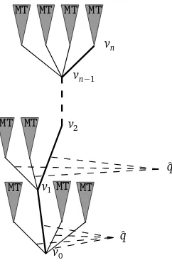
Proof :We consider the setT∗of trees with a marked path from the root, that is, an element ofT∗ is of the form(T,v0,v1, ...), whereT is inT,v0=eandvi=←−−vi+1.
We consider the filtrationFk=σ(T,v1, ...vk). Given an integern, we introduce the lawdMT∗nonT∗
de-fined as follows : we consider a vertexe(the root), to this vertex we attach a set of marked children with lawˆq, and we chose one of those children as v1, with probabilityP(x =v1) =A(x)/
P
A(ei). To each child ofedifferent fromv1we attach independently a tree with lawMT, and onv1we iterate
the process : we attach a set of children with lawqˆ, we choose one of these children to bev2, and so on, until getting to the leveln. Then we attach a tree with lawMTtovn.
ˆ q
MT MT MT
v0
v1
ˆ q
MT MT v2
vn−1
vn
MT MT MT MT
Figure 3: the lawMTd∗
n.
The same calculations as in the proof of Lemma 3.2 allow us to see the following fact : for f Fn-measurable,
EdMT∗ n
[f(T,v0, ...,vn)] =EMT
X
x∈Tn
Cxf(T,p(x))
, (10)
where p(x) is the path from eto x. Note that, by construction, under MTd∗n conditionally to ˜Fn∗ := (Cvi, 0≤i≤n), the trees T
(vi), 0≤i≤nof the descendants of v
i who are not descendants ofvi+1
are independent trees, and the law ofT(vi)is the law of a MTtree, except for the first level, whose
law isˆqconditioned onvi+1,A(vi+1).
For a tree T inT∗we have
Wv
k =
X
vk=←−x,x6=vk+1
A(x)Wx+A(vk+1)Wv
k+1:=W
∗
k +A(vk+1)Wvk+1,
where
Wj∗= lim
n→∞
X
x∈T,vj<x,vj+16≤x,d(vj,x)=n Y
v≤z≤x
A(z).
Iterating this, we obtain
Wvk =
n−1 X
j=k
Wj∗
j
Y
i=k+1
A(vi) +Wvn
n
Y
i=k+1
with the convention that the product over an empty space is equal to one. We shall use the notation
Ai:=A(vi)for a tree with a marked ray.
Finally, summing over k, we obtain
Svn=
where, conditionally to theAi, Ui are i.i.d. random variables, with the same law asMn. We get
EMT[(Mn+1−1)2] =ρ(2)EMT[(Mn−1)2] +C2,
where C2 is a finite number. It is easy to see then that E[Mn2]is bounded, and martingale theory implies that Mn converges in L2. Using the fact that EMTd∗n[Wvk] =EØMT∗ for n large enough
Inequality from page 82 of[22]implies
where we have admitted the following lemma
Lemma 4.3. ∀µ < κ,there exist some constant C such that
moreover, there exists someǫ1>0such that
EMT∗ n[W
∗
i |F˜n∗]> ǫ1.
We postpone the proof of this lemma and finish the proof of Lemma 4.2. In order to boundEdMT∗
Bλi
we need to introduce a result from[4](lemma 4.1).
Statement 4.1(Biggins and Kyprianou). For any n≥1and any measurable function G,
EMT
where Sn is the sum of n i.i.d variables whose common distribution is determined by
E[g(S1)] =Eq
for any positive measurable function g.
In particular,E[eλS1] =E
Using Minkowski’s Inequality, we get
EMTd∗
We can now conclude,
En(1)≤C5nλ/2,
and by Markov’s Inequality,
P1<C6/(ελnλ/2). (14)
Now we are going to deal with
Lemma 4.3 implies that Ed
MT∗n[W
∗
j|F˜n∗] is bounded above and away from zero, and a deterministic function ofAj+1. We shall note accordingly
Ed
MT∗n[W
∗
j|F˜n∗]:=g(Aj+1). (15)
Recalling (11), we have
EMTd∗ n
[Svn|F˜
∗
n] = n
X
j=0
EMTd∗ n
[Wj∗|F˜n∗])Bj=
X
0≤j≤k≤n k
Y
i=j
Aig(Ak+1).
with the conventiong(An+1) =1 andA0=1. We set accordingly
Ed
MT∗n[Svn|F˜
∗
n]:=F(A1, ...,An).
Recalling that, due to Statement 4.1, under the lawMTd∗
n, theAi are i.i.d random variables we get
EdMT∗ n
[F(A1, ...,An)] =
X
0≤j≤k≤n k
Y
i=j
EMTd∗ n
[Ai]EMTd∗n[g(Ak+1)].
Form≥0 we call
Fm[Am+1, ...,An]
:= X
0≤j≤k≤n k≤m−1
k
Y
i=j
EMTd∗ n
[Ai]EdMTn∗[g(Ak+1)] +
X
0≤j≤k≤n k≥m
m
Y
i=j
EMTd∗ n
[Ai] k
Y
i′=m+1
Ai′g(Ak+1).
Note thatF0=F andFn=Ed
MT∗n[Svn], thus we can write
Ed
MT∗n[Svn|F˜
∗
n]−EMTd∗n[Svn] =F 0(A
1, ...An)−Fn
=F0(A1, ...An)−F1(A2, ...An)
+F1(A2, ...An)−F2(A3, ...An)....
+Fn−1(An)−Fn.
We introduce the notations ρ := EMTd∗ n
[A1] = ρ(2) < 1, and for a random variable X, ˜X := X −
Ed
The last expression gives us
We deduce easily that
whereC7,C8 are finite constants and
Dk=
Markov’s Inequality then implies
On the other hand, we call for 0≤k≤n, We can compute the quadratic variation of this martingale
〈Nk〉:=
On the other hand, the total quadratic variation ofNk is equal to
[Nk]:=
It is easy to check that if the event in (18) is fullfilled, then there exists some constantC12such that
〈Nk〉<C12n
Putting together (14) and (19), we obtain (9). This finishes the proof of Lemma 4.2. In particular, ifκ >5, we can chooseλ >4, so that
EMT[X
x∈Aε
n
Cx]<n−µ,
withµ >1 . The following corollary is a direct consequence of the proof.
Corollary 4.4. For every a>0and2< λ < κ−1,
Pd
MT∗n[|Svk−kη|>a]≤C1
k1−λ/2
aλ .
Note that the upper bound is trivial under assumption (3). We suppose (H2), Let f be a measurable test function, we have by construction
Eˆq
By standard convexity property, we get that the last term is lesser or equal to
∞ while, still by construction
Eqˆ
We have
Let us go back toIMTtrees. We consider the following sets
Bεn=
We can now prove the following
Lemma 4.5.
andIMTalmost surely, for someε,
Since Mt is a martingale with bounded normalized quadratic variation Vt, we get that, for IMT
almost every treeT,
PT(Γt)→0.
Going back to our initial problem, we have
PT(Xρ part of the right hand term of (23) is equal to
1
Lemma 4.2 implies that, underIMTconditioned on{Ray,A(vi)},Ni are independent and identically distributed variables, with finite expectation, up to a bounded constant due to the first level of those
subtrees. We are now going to computeETP Hv follows a geometric law, with parameterpi=Pvi
T[Hv⌊tγ⌋<Hvi].
Standard computations for random walks onZ, (see, for example, Theorem 2.1.12 of[24]) imply that
pi= ω(vi,vi+1)
1+P⌊j=tγi⌋−1Qk⌊=tγ⌋j−1A(vk) ,
and, going back to our initial problem,
Markov’s Inequality and the Borel Cantelli Lemma imply that,IMT-almost surely, there existst0such that∀t>t0,Vt≤tµ, and then,
PT(Xρt ∈ ∪
∞
n=1B
ε
m)≤PT(Γt) +
C16
⌊tδ−µ⌋
⌊tγ⌋ X
i=0
Ni.
Sinceδ−µ < γ, an application of the law of large numbers finishes the proof of Lemma 4.5.
We are now able to prove the first part of Proposition 4.2. Note that underIMT,Sv
nfollows the same
law asSvnin aT
∗tree underdMT∗
n, whence
Svn/nn→→∞−η
in probability. LetQt be the first ancestor ofXρt onRay. Statement 4.1 and standard RWRE theory
imply thatQt is transient, therefore
SQt/h(Qt)t→∞→ η,
so that, for any positiveε1, for large t,
|SQt/η−h(Qt)| ≤ε1sup
s≤2t|
Mt|. (25)
We can now compute
|Mρ
t/η−h(Xρt)|=|S
Ray
Xρt/η−d(Xρt,Ray) +SQt/η−h(Qt)|.
In view of (25) on the event{Xρt 6∈ ∪
∞
n=1B
ε
m}, we have
|Mρt/η−h(Xρt)| ≤2ε1sup
s≤2t|
Ms|.
The processVt being boundedIMTa.s., a standard martingale inequality implies
lim
ε1→0
lim sup t→∞
P0 T(sup
s≤t |
Ms|> εpt/(2ε1)) =0.
It follows that
lim
t→∞PT(|Mρt/η−h(Xρt)| ≥ε
p
t) =0,IMT−a.s.
We are now going to prove the second part of Proposition 4.2. The course of the proof is similar to [21]. We have the following lemma
Lemma 4.6. for any u, t≥1,
P
MT(|Xi| ≥u for some i≤t)≤2t e−u
2/2t
.
Proof :We consider the graphT∗obtained by truncating the treeTafter the levelu−1, and adding an extra vertex e∗, connected to all vertices in Tu−1. We construct a random walk Xs∗ on T∗ as following
P0
T(Xi∗+1= y|Xi∗=x) =
ω(x,y)if|x|<u−1 or|x|=u−1,|y|=u−2
1−ω(x,←−x)if|x|=u−1,y=e∗
˜
ω(e∗,y)if x=e∗,|y|=u−1
We can choose ˜ω(e∗,y) arbitrarily, provided Py∈T
u−1ω˜(e
∗,y) = 1, so we will use this choice to
ensure the existence of an invariant measure : indeed, ifπis an invariant measure for the walk, one can easily check that, for anyx such that|x| ≤u−1, callingx(1)the first vertex on the path frome
tox,
π(x) = π(e)ω(e,x
(1))
ω(x,←−x)
Y
x(1)<z≤x
A(z).
Further, we need that, for everyx ∈Tu−1,
π(x)(1−ω(x,←x−)) =π(e∗)ω˜(e∗,x). Summing over x, and usingPy∈T
uω˜(e
∗,y) =1, we get
π(e∗) =π(e) X x∈Tu−1
ω(e,x(1)) Y x(1)<z≤x
A(z)
P
ω(x,xi)
ω(x,←x−)
≤π(e)X x∈Tu
Y
x(1)<z≤x
A(z)≤π(e)Yu.
Then,
P
MT(∃i≤t,Xi≥u)≤PMT(∃i≤t,X∗i =e∗)≤ t
X
i=1
P
MT(Xi∗=e∗). By the Carne-Varnopoulos Bound (see[17], Theorem 12.1),
PT(X∗i =e∗)≤2pYue−u
2/2i
.
Since, by Jensen’s Inequality,EMT(pYn)≤1,
P
MT(Xi≥ufor somei≤t)≤2t e−u
2/2t
.
We have the following corollary, whose proof is omitted
Corollary 4.7.
P
IMT(|h(Xi)| ≥u for some i≤t)≤4t3e−(u−1)
2/2t
.
Proof : see[21], Corollary 2.
We can now finish the proof of the second part of Proposition 4.2. Under PIMT, the increments
h(Xi+1)−h(Xi)are stationnary, therefore, for anyεandr,s≤t with|s−r| ≤tδ,
PIMT(|h(Xr)−h(Xs)| ≥t1/2−ε)≤PIMT(|h(Xr−s)| ≥t1/2−ε)≤4t3e−t
1−δ−2ε .
Whence, by Markov’s Inequality, for all t large,
PIMTP0
T
|h(Xr−s)| ≥t1/2−ε≥e−t1−δ−ε≤e−t1−δ−ε. Consequently,
PIMT P0T sup
r,s≤t,|r−s|≤tδ|
h(Xr)−h(Xs)| ≥t1/2−ε
!
≥e−t1−δ−ε
!
The Borel-Cantelli Lemma completes the proof.
We are now able to finish the proof of Theorem 4.1. Due to Proposition 4.1, the process
{M⌊nt⌋/pσ2η2n} converges, for IMT almost every T, to a standard Brownian motion, as n goes
to infinity. Further, by Theorem 14.4 of[5],{Mρnt/
p
σ2η2n}converges, forIMTalmost every T, to
a standard Brownian motion, asngoes to infinity. Proposition 4.2 implies that the sequence of
pro-cesses{Ytn}={h(Xρ
nt)/ p
σ2n}is tight and its finite dimensional distributions converge to those of
a standard Brownian motion, therefore it converges in distribution to a standard Brownian motion, and, applying again Theorem 14.4 of[5], so does{h(X⌊nt⌋/
p σ2n}.
5
Proof of Theorem 1.2.
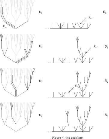
In this section we finish the proof of Theorem 1.2. Our argument relies on a coupling between random walks onMTand onIMTtrees, quite similar to the coupling exposed in[21]. Let us introduce some notations : forT,S two trees, finite or infinite, we set LT the leaves of T, that is the vertices of T that have no offspring, To = T/LT and for v ∈T we denote by T◦vS the tree obtained by gluing the root ofS to the vertex v ofT, with vertices marked as in their original tree (the vertex coming from bothvand the root ofSis marked asv). Given a treeT ∈Tand a path{Xt}on T we construct a family of finite trees Ti,Ui as follows : letτ0=η0=0, andU0 the finite tree consisting
of the rooteofT and its offspring, marked as in T. Fori≥1, let
τi=min{t≥ηi−1:Xt ∈LUi−1} (26) ηi=min{t> τi;Xt ∈Uio−1}. (27)
LetTi be the tree “explored” by the walk during the excursion[τi,ηi), that is to sayTi is composed of the vertices of T visited by{Xt,t ∈[τi,ηi)}, together with their offspring, marked as in T, and the root ofTi isXτi. LetUi =Ui−1◦
Xτ
i Ti be the tree explored by the walk from the beginning. We
call{uit}ηi−τi−1
t=0 the path inTi defined byuit = Xτi+t. If T is distributed according toMT, andXt is
the path of the random walk onT, then, the walk being recurrent,P
MT−almost surelyT =limUi.
We are now going to construct ˜T ∈ T˜, a tree with a semi-infinite ray emanating from the root, coupled with T, and a path{X˜t}on T, in such a way that, if T is distributed according to MT, and
Xt is the path of the random walk on T, then ˜T will be distributed according to IMTand{X˜t}will follow the law of a random walk on ˜T.
Let ˜Uo be the tree defined as follows : we choose a vertex denoted bye, as the root of ˜Uo, and a semi-infinite ray{e= v0,v1, ...}. To each vertex vi ∈Ra y different fromewe attach independently a set of marked vertices with lawqˆ. To ewe attach a set of children with distribution(q+ ˆq)/2 If
i≥1 we chose one of those vertices, with probability PA(x)
yA(y)
, and identify it withvi−1. We obtain a tree with a semi-infinite ray and a set of children for each vertexvi onRa y, one of them beingvi−1. We set ˜τ0=η˜0=0. Recalling the relation (5) between theAx and theω(x,y), one can easily check that for any vertexx, knowing the{w(x,y)}y∈T is equivalent to knowing{A(xi)}xichildren ofx. Thus, knowing ˜U0 one can compute the{ω(x,y)}x∈Ra y,y∈U˜0and define a random walk ˜Xt on ˜U0, stopped
˜
U0
U0
U1
b
˜
Xτ1
˜
U1
˜
U2
˜
Xτ2
b
˜
Xτ3
b
U2
˜
U3 U3
Xn
We are now going to “glue” the first excursion of{Xt}. Let
˜
U1=U˜0◦X˜τ˜1 T
1,
˜
η1=τ˜1+η1−τ1,
{X˜t}η˜1−1
t=τ˜1 =u
1
t−τ˜1,
˜
Xη˜1=←−−−X˜η˜1−1.
One can easily check that{X˜t}t≤η˜1 follows the law of a random walk on ˜U1.
We iterate the process, in the following way : fori>1, start a random walk{X˜t}t≥η˜
i−1on ˜Ui−1, and
define
˜
τi=min{t>0 : ˜Xt∈LU˜i−1},
˜
Ui=U˜i−1◦X˜˜τi T
i, ˜
ηi=τ˜i+ηi−τi,
{X˜t}η˜i−1
t=τ˜i =u
i t−τ˜i,
˜
Xη˜i =←−−−X˜η˜i−1.
Finally, set ˜U =S∞0 U˜iand ˜T the tree obtained by attaching independentsMTtrees to each leaves of ˜
U. It is a direct consequence of the construction that
Proposition 5.1. If T is distributed according toMTand XtfollowsPT, thenT is distributed according˜
toIMT, andX˜tfollowsPT˜.
As a consequence, under proper assumptions onq, application of Proposition 4.1 implies that forMT
almost everyT the process{h(X˜⌊nt⌋)/pσ2n}converges to a standard Brownian motion, asngoes
to infinity.
We introduceRt=h(X˜t)−minit=1h(X˜i). We get immediately that
{R⌊nt⌋/ p
σ2n}converges to a Brownian motion reflected to its minimum, which has the same law
as the absolute value of a Brownian motion.
In order to prove Theorem 1.2, we need to control the distance betweenRt and|Xt|.
Let It = max{i: τi ≤ t} and ˜It =max{i : ˜τi ≤ t} the number of excursions started by {Xt}and
{X˜t}before time t. Let∆t =PIt
i=1(τi−ηi−1)and ˜∆t =
P˜It
i=1(τ˜i−η˜i−1), which measure the time
spent by{Xt}and{X˜t}outside the coupled excursions before timet. By construction, the distance betweenRt and|Xt| comes only from the parts of the walks outside those excursion. In order to control these parts, we set for 0≤α <1/2
∆αt = It X
i=1
τXi−1
s=ηi−1
1|Xs|≤tα;
similarly,
˜ ∆αt =
˜
It X
i=1 ˜
τXi−1
s=η˜i−1