Solvable Rational Potentials
and Exceptional Orthogonal Polynomials
in Supersymmetric Quantum Mechanics
⋆Christiane QUESNE
Physique Nucl´eaire Th´eorique et Physique Math´ematique, Universit´e Libre de Bruxelles, Campus de la Plaine CP229, Boulevard du Triomphe, B-1050 Brussels, Belgium
E-mail: [email protected]
Received June 12, 2009, in final form August 12, 2009; Published online August 21, 2009 doi:10.3842/SIGMA.2009.084
Abstract. New exactly solvable rationally-extended radial oscillator and Scarf I potentials are generated by using a constructive supersymmetric quantum mechanical method based on a reparametrization of the corresponding conventional superpotential and on the addition of an extra rational contribution expressed in terms of some polynomialg. The cases where
g is linear or quadratic are considered. In the former, the extended potentials are strictly isospectral to the conventional ones with reparametrized couplings and are shape invariant. In the latter, there appears a variety of extended potentials, some with the same charac-teristics as the previous ones and others with an extra bound state below the conventional potential spectrum. Furthermore, the wavefunctions of the extended potentials are con-structed. In the linear case, they contain (ν+ 1)th-degree polynomials with ν = 0,1,2, . . ., which are shown to beX1-Laguerre orX1-Jacobi exceptional orthogonal polynomials. In the quadratic case, several extensions of these polynomials appear. Among them, two different kinds of (ν+ 2)th-degree Laguerre-type polynomials and a single one of (ν + 2)th-degree Jacobi-type polynomials withν= 0,1,2, . . .are identified. They are candidates for the still unknownX2-Laguerre andX2-Jacobi exceptional orthogonal polynomials, respectively.
Key words: Schr¨odinger equation; exactly solvable potentials; supersymmetry; orthogonal polynomials
2000 Mathematics Subject Classification: 33E30; 81Q05; 81Q60
1
Introduction
Since the pioneering work of Bargmann [1], there has been a continuing interest in generating rational potentials for which the Schr¨odinger equation is exactly or quasi-exactly solvable. In this respect, supersymmetric quantum mechanics (SUSYQM) [2,3,4,5,6], as well as the related intertwining operator method [7] and the Darboux algorithm [8], have attracted considerable attention (see, e.g., [9,10,11,12,13,14,15,16]).
SUSYQM indeed provides us with a powerful technique for designing Hamiltonians with a prescribed energy spectrum from some known exactly solvable one. For one-dimensional systems, to which we are going to restrict ourselves here, the simplest approach based upon first-order intertwining operators uses a single solution of the initial Schr¨odinger equation, defining the so-called superpotential. The latter then furnishes a SUSY partner Hamiltonian, whose spectrum may differ by at most one level from that of the initial Hamiltonian. More flexibility may be achieved by resorting tonth-order intertwining operators withn >1, constructed fromn
⋆This paper is a contribution to the Proceedings of the Eighth International Conference “Symmetry in Nonlinear Mathematical Physics” (June 21–27, 2009, Kyiv, Ukraine). The full collection is available at
solutions of the initial Hamiltonian [17, 18, 19, 20, 21, 22, 23]. These higher-order operators may turn out to be reducible into a product of lower-order ones or to be irreducible.
In all cases, not only the SUSY partner potential and spectrum are explicitly known, but also the corresponding wavefunctions are given by some analytic formulae. The resulting expressions for the potential and the eigenfunctions, however, often look a good deal more complicated than those for the initial Hamiltonian (see, e.g., [24]). In such a context, to get a SUSY partner potential that is some rational function is not a simple task in general.
An efficient method for getting potentials and wavefunctions expressed in terms of some elementary functions was proposed a few years ago and called algebraic Darboux transforma-tion [14, 15]. This procedure, whose idea goes back to an older paper [25], consists in using the solutions of the hypergeometric or confluent hypergeometric function whose log derivative is a rational function and which have been classified by mathematicians [26].
In a recent work [27], an alternative scheme has been devised. Known exactly solvable potentials are rationally extended by effecting a reparametrization of the starting Hamiltonian and redefining the existing superpotential in terms of modified couplings, while allowing for the presence of some rational function in it. The newly introduced parameters can be adjusted in such a way that the initial exactly solvable potential with reparametrized couplings becomes isospectral to a superposition of the same (but with its parameters left undisturbed) and some additional rational terms. Such a first-order SUSY transformation has been shown to be part of a reducible second-order one, which explains the isospectrality of the conventional and rationally-extended potentials with the same parameters.
The purpose of the present paper is twofold: first to demonstrate the efficiency of this method in producing rather complicated exactly solvable rational potentials, whose existence would otherwise have remained unknown, and second to examine in some detail the polynomials appearing in the rational potential bound-state wavefunctions. Among these polynomials, the simplest ones belong to two classes of exceptional orthogonal polynomials, which have been the topic of some recent mathematical study [28, 29]. We plan to show here that our SUSYQM approach provides us with a convenient way of constructing and generalizing such polynomials. This paper is organized as follows. In Section 2, the method is first applied to rationally extend the radial oscillator potential and to study the associated Laguerre-type polynomials. The generalization to the Scarf I potential and to the corresponding Jacobi-type polynomials is then dealt with in Section 3. Finally, Section4 contains some final comments.
2
Radial oscillator potential
The radial oscillator potential
Vl(x) = 1 4ω
2x2+l(l+ 1)
x2 , (2.1)
where ω and l denote the oscillator frequency and the angular momentum quantum number, respectively, is defined on the half-line 0 < x < ∞. It supports an infinite number of bound states, whose energies are given by
Eν(l)=ω 2ν+l+32
, ν = 0,1,2, . . . . (2.2)
The associated wavefunctions, vanishing at the origin and decaying exponentially at infinity, can be expressed in terms of Laguerre polynomials as [3,30]
ψ(νl)(x) =Nν(l)xl+1L (l+1
2) ν (z)e−
1 4ωx
2
, z≡ 1 2ωx
where
Nν(l)= ω
2
12(l+32) 2ν!
Γ(ν+l+32)
!1/2
.
Before applying SUSYQM to such a potential, let us briefly review some well-known proper-ties of this method [2,3,4,5,6].
In the minimal version of SUSY, one considers a pair of first-order differential operators
ˆ
A= d
dx+W(x), Aˆ †=
−dxd +W(x), (2.4)
and a pair of factorized Hamiltonians
H(+)= ˆA†Aˆ=− d 2
dx2 +V
(+)(x)−E, H(−)= ˆAAˆ†=− d2 dx2 +V
(−)(x)−E, (2.5)
where E is the so-called factorization energy. To E one can associate a factorization func-tion φ(x), such that H(+)φ(x) = Eφ(x). The superpotential is given in terms of φ(x) by the relationW(x) =−φ′(x)/φ(x) and the two partner potentialsV(±)(x) are connected withW(x)
through the equation
V(±)(x) =W2(x)∓W′(x) +E, (2.6)
where a prime denotes derivative with respect to x.
Whenever E and φ(x) are the ground-state energy E0(+) and wavefunction ψ0(+)(x) of the initial potential V(+)(x), i.e., H(+)φ(x) = H(+)ψ(+)
0 (x) = 0, the partner potential V(−)(x)
has the same bound-state spectrum as V(+)(x), except for the ground-state energy which is removed (casei). ForE < E0(+), in which caseφ(x) is a nonnormalizable eigenfunction ofH(+), the partnerV(−)(x) has the same spectrum asV(+)(x) ifφ−1(x) is also nonnormalizable (caseii)
or has an extra bound-state energyE belowE0(+), corresponding to the wavefunctionφ−1(x), if
the latter is normalizable (case iii).
The standard SUSY approach to the radial oscillator potential corresponds to casei. Deletion of the ground-state energyE0(l)yields a partner potentialVl+1(x) of the same kind, this meaning
that the radial oscillator potential is shape invariant [31]. In this case,φ(x) =xl+1exp(−1 4ωx2)
or, in other words,
W(x) = 1 2ωx−
l+ 1
x . (2.7)
We now plan to modify such a superpotential in order to generate rationally-extended radial oscillator potentials.
2.1 Extended classes of rational radial oscillator potentials
Motivated by the form of the standard superpotential (2.7) and by the fact that z = 12ωx2 is
the basic variable appearing in the Laguerre polynomials that control the bound-state wave-functions (2.3), let us make the ansatz
W(x) =ax+ b
x− dg/dx
g , (2.8)
such a way that V(+)(x), as defined in (2.6), continues to belong to the radial oscillator family up to some change in l, while its partner V(−)(x) differs from V
l(x) in the presence of some additional rational terms, i.e.,
V(+)(x) =Vl′(x), V(−)(x) =Vl,ext(x) =Vl(x) +Vl,rat(x).
To be physically acceptable, such additional terms Vl,rat(x) must be singularity free on the
half-line 0< x <∞.
In the following, we carry out this programme for linear and quadratic polynomialsg(x2).
2.1.1 Linear case
Let us assume that
g(x2) =x2+c, dg(x 2)
dx = 2x,
where c is a constant satisfying the condition c > 0 in order to ensure the absence of poles on the half-line.
On inserting the ansatz (2.8) in (2.6), we obtain
V(+)(x) =a2x2+b(b+ 1)
x2 + 2
2(ac−b) + 1
x2+c +a(2b−5) +E.
Elimination of the term proportional to (x2+c)−1 and of the additive constant from V(+)(x)
can be achieved by choosing
c= 2b−1
2a , E =−a(2b−5).
The partner potential is then given by
V(−)(x) =V(+)+ 2W′ =a2x2+b(b−1)
x2 +
4
x2+c −
8c
(x2+c)2 + 2a
and its first two terms coincide with Vl(x), defined in (2.1), if the two conditions
a2= 14ω2, b(b−1) =l(l+ 1)
are fulfilled. These two restrictions lead to four possible solutions for (a, b): (a, b) = ω2, l+ 1
, ω
2,−l
, −ω2, l+ 1
, −ω2,−l
.
As a result, c becomes c = ±(2l+ 1)/ω, where only the upper sign is allowed. Since this is achieved either for (a, b) = ω2, l+ 1
or for (a, b) = −ω2,−l
, we arrive at two distinct solutions1,
V(+)(x) =Vl±1(x), V(−)(x) =Vl(x) +
4ω
ωx2+ 2l+ 1−
8ω(2l+ 1)
(ωx2+ 2l+ 1)2 ±ω, (2.9)
corresponding to
W(x) =±1 2ωx±
l+12 ±12
x −
2ωx
ωx2+ 2l+ 1, (2.10)
E =−ω l+12 ∓2
, (2.11)
φ(x) =x∓(l+12)− 1
2(ωx2+ 2l+ 1)e∓ 1 4ωx
2
, (2.12)
1
where we take either all upper or all lower signs, respectively. We can therefore go from a con-ventional radial oscillator potential to an extended potential Vl,ext(x) in first-order SUSYQM
provided we start either from Vl+1(x) or from Vl−1(x) and, apart from some irrelevant additive
constant, the result of the extension is the same in both cases.
Since the factorization energy E, given in (2.11), is smaller than the ground-state energy of V(+)(x), namely E0(l±1) = ω l+32 ±1
, it is clear that we must be in case ii or case iii of SUSYQM. On examining next the behaviour of the factorization function, it becomes apparent that it is the former case that applies here, namelyV(+)(x) andV(−)(x) are strictly isospectral. We indeed observe that for the first choice corresponding to upper signs in (2.12), φ decays exponentially for x→ ∞, but grows as x−l−1 forx→0, while for the second choice associated
with lower signs, it vanishes for x→0, but grows exponentially forx→ ∞.
We conclude that the addition of the two rational terms 4ω(ωx2 + 2l+ 1)−1 and −8ω(2l+ 1)(ωx2+ 2l+ 1)−2 toVl(x) has not changed its spectrum, which remains given by equation (2.2).
2.1.2 Quadratic case
For
g(x2) =x4+cx2+d, dg(x 2)
dx = 2x(2x 2+c),
where c and d are two constants, the picture gets more involved because the singularity-free character of the extended potential on the half-line can be ensured in two different ways: the quadratic polynomialg(x2) may have either two real and negative roots or two complex conjugate ones. In association with these two possibilities, we will have to distinguish between the two cases
c >0, 0< d≤ c 2
4, (2.13)
and
d > c 2
4. (2.14)
On proceeding as in the linear case, it is straightforward to get
V(+)(x) =a2x2+b(b+ 1)
x2 + 2
2(ac−2b+ 3)x2+ 4ad−(2b−1)c
x4+cx2+d +a(2b−9) +E,
leading to the conditions
c= 2b−3
a , d=
(2b−1)(2b−3)
4a2 , E =−a(2b−9).
Furthermore
V(−)(x) =a2x2+b(b−1)
x2 +
4(2x2−c)
x4+cx2+d+
8(c2−4d)x2
(x4+cx2+d)2 + 2a
yields the same four possibilities for (a, b) as before. To go further, we have to distinguish between (2.13) and (2.14).
In the real case, the condition c > 0 can be achieved by imposing a = 12ω, b = l+ 1 with
to (2b−1)/a > 0, discards the choice a = −21ω, b = 1. Finally, d ≤ c42 turns out to impose
a <0. Hence we are left with a single solution corresponding to
a=−1
As a result, we get for l >0 the pair of partner potentials
V(+)(x) =Vl−1(x),
Turning ourselves to the complex case, we observe that the single conditiond > c42 is equiv-alent to b > 32, which imposes b=l+ 1 with l >0. The sign ofa remaining undetermined, we have actually here two distinct solutions according to the choice made, namely
a=±1
In comparison with the linear case which has provided us with a single rationally-extended potential, the quadratic one reveals itself much more flexible since three distinct rationally-extended potentials with l >0 have been obtained. It is also worth observing that the angular momentuml′ of the starting potential has now a strong influence on the resulting extended one.
Furthermore, we note that in all three cases, the factorization energy is smaller than the ground-state energy of V(+)(x), as in the linear case. As far as the factorization function is concerned, however, a distinction must be made between the function in (2.16) or that with upper signs in (2.18), on one hand, and that with lower signs in the latter equation, on the other hand. For the first two functions, the situation is similar to the previous one leading to strictly isospectral partner potentials (case ii), whereas, for the third function, we observe that
φ−1(x) is normalizable on the half-line and is therefore the ground-state wavefunction of the
correspondingV(−)(x) potential with an energy eigenvalueE(−)
0 =E
(l+1)
0 −6ω=ω l−72
2.2 Determination of wavefunctions
The factorized forms (2.5) of H(+) and H(−) imply the existence of the intertwining relations [2,3,4,5,6]
H(+)Aˆ†= ˆA†H(−), AHˆ (+)=H(−)A,ˆ
which enable us to determine the wavefunctions of H(−) from those of H(+) with the same energy (or vice versa). Hence, on starting from H(+)ψν(+)(x) =ενψν(+)(x) with εν =E(l
according to whether caseii or case iiiof SUSYQM applies.
We will now proceed to use equations (2.19) and (2.20) to determine the wavefunctions of the rationally-extended radial oscillator potentials constructed in Section 2.1.
2.2.1 Linear case choice. On applying this operator on the right-hand side of equation (2.3) withl−1 substituted forl, and employing equation (2.19), we get
The partner potential wavefunctions (2.21) can therefore be expressed in terms of ˆL(να+1) (z) as
ψ(−)ν (x) =Nν(−)
xl+1 ωx2+ 2l+ 1Lˆ
(l+1 2) ν+1 12ωx
2 e−14ωx
2
, (2.23)
where
Nν(−)=
ωl+32ν!
2l−32 ν+l+3 2
Γ ν+l+12 !1/2
.
Similarly, for the other choiceψ(+)ν (x) =ψν(l+1)(x), we can write
ψ(−)ν (x) = √4
ενN (+) ν
xl+1e−14ωx 2
ωx2+ 2l+ 1Oˆ (α)
2 L(να+1)(z),
where Nν(+)=Nν(l+1),εν = 2ω ν+l+12,α=l+12, and
ˆ
O2(α)≡(z+α)
z d
dz +α+ 1
−z.
On taking into account that this time
ˆ
O2(α)L(να+1)(z) =−(ν+α) ˆL(να+1) (z),
we arrive (up to some irrelevant overall sign) at the same wavefunctions (2.23) as in the previous derivation, as it should be.
At this stage, some observations are in order. In [28, 29], it has been shown that the family of (ν+ 1)th-degree polynomials ˆL(να+1) (z), ν = 0,1,2, . . ., defined in equation (2.22), arises in a natural way when extending Bochner’s theorem on the relations between classical orthogonal polynomials and solutions of second-order eigenvalue equations [33] by dropping the assumption that the first element of the orthogonal polynomial sequence be a constant. It is actually one of the two complete orthogonal sets of polynomials with respect to some positive-definite measure that can be constructed by starting instead with some linear polynomial (the second one being considered in Section 3.2). For this reason, the exceptional polynomials ˆL(να+1) (z) have been called X1-Laguerre polynomials [28,29]. They satisfy a second-order eigenvalue equation
with rational coefficients and are normalized in such a way that their highest-degree term is equal to (−1)ν+1zν+1/ν! (as compared with (−1)νzν/ν! for L(να)(z)). On combining their definition (2.22) with the recursion relation of classical Laguerre polynomials, one can write them as linear combinations of three Laguerre polynomials with constant coefficients,
ˆ
Lαν+1(z) = (ν+ 1)Lαν+1(z)−2(ν+α+ 1)Lαν(z) + (ν+α+ 1)Lαν−1(z). (2.24)
A first few polynomials are listed in Appendix A, where they may be contrasted with the corresponding classical Laguerre ones.
The extended radial oscillator potential (2.9) and its corresponding wavefunctions (2.23) were derived for the first time in [34] by using the point canonical transformation method [35] and the differential equation satisfied by ˆL(να+1) (z). In the same work, the potential was also shown to be shape invariant with a partner given by Vl+1,ext(x). Here we have adopted another type
2.2.2 Quadratic case
As proved in Section 2.1.2, the quadratic case leads to three distinct new rationally-extended potentials, of which the first two are similar to that obtained in the linear case (case ii of SUSYQM), while the third one is not (caseiii of SUSYQM).
By proceeding as in the linear case and definingz = 12ωx2 and α =l+ 12, we arrive at the
leading to three distinct families of Laguerre-type polynomials,
˜
for cases I, II, and III, respectively.
The corresponding rationally-extended potential wavefunctions can be written as
Let us examine in more detail the Laguerre-type polynomials obtained in the first two cases. From physical considerations related to general properties of SUSYQM, it follows that the wavefunctions ψ(−)ν (x), ν = 0,1,2, . . ., form two complete, orthonormal sets in the Hilbert spaces associated with the corresponding rationally-extended potentials. This suggests that a similar property should be valid for ˜L(1α,ν)+2(z) and ˜L(2α,ν)+2(z) with respect to some appropriate positive-definite measure. From the additional fact that the lowest-degree polynomials are quadratic inz (see AppendixA), we infer that ˜L(1α,ν)+2(z) and ˜L(2α,ν)+2(z) are good candidates for the still unknown X2-Laguerre polynomials. Note also that by analogy with classical andX1
-Laguerre polynomials, in defining them in (2.25) and (2.26), we have chosen their normalization in such a way that their highest-degree term is equal to (−1)ν+2zν+2/ν!. Furthermore, it is straightforward to show that the counterparts of equation (2.24) are now linear combinations of five Laguerre polynomials with constant coefficients,
˜
L(1α,ν)+2(z) = (ν+ 2)(ν+ 1)L(να+2) (z)−4(ν+ 1)(ν+α+ 2)L(να+1) (z)
+ 2(ν+α+ 2)(3ν+ 2α+ 2)L(να)(z)−4(ν+α+ 2)(ν+α)L(να−1)(z)
+ (ν+α+ 2)(ν+α−1)L(να−2) (z)
and
˜
L(2α,ν)+2(z) = (ν+ 2)(ν+ 1)L(να+2) (z)−4(ν+ 1)(ν+α+ 1)L(να+1) (z)
+ 2(ν+α+ 1)(3ν+ 2α+ 1)L(να)(z)−4(ν+α+ 1)(ν+α)L(να−1)(z)
+ (ν+α+ 1)(ν+α)L(να−2) (z).
Since for case III, the wavefunctions ψν(−)+1(x) have to be supplemented with the function
φ−1(x) in order to form a complete set of orthonormal wavefunctions for the corresponding
rationally-extended potential (see equation (2.20)), it is rather clear that the Laguerre-type polynomials ˜L(3α,ν)+3(z) will not form a complete orthogonal set of exceptional polynomials. One of their properties is however worth pointing out. Although from their definition (2.27) one would expect that their expansion in terms of classical Laguerre polynomials would contain seven terms, one actually gets only five of them, i.e.,
˜
L(3α,ν)+3(z) = (ν+ 2)(ν+ 1)L(να+3) (z)−4(ν+ 2)(ν+ 1)L(να+2) (z)+ 2(ν+ 1)(3ν+α+ 5)L(να+1) (z)
−4(ν+ 1)(ν+α+ 1)L(να)(z) + (ν+α+ 1)(ν+α)L(να−1) (z),
the coefficients ofL(να−2) (z) andL(να−3) (z) vanishing identically. Observe that in (2.27), the polyno-mials have been normalized in such a way that their highest-degree term is (−1)ν+3zν+3/[(ν+ 3)ν!].
In cases I and II, the extended potential ground-state wavefunction ψ(−)0 (x), expressed in
terms of ˜L(l+ 1 2) 1,2 12ωx2
or ˜L(l+ 1 2) 2,2 12ωx2
, respectively, can be used to prove that the correspon-ding potentialVl,ext(x) is shape invariant, its partner being given byVl+1,ext(x) (see AppendixD).
This generalizes to the quadratic case a property already demonstrated for the linear one in [34].
3
Scarf I potential
The Scarf I potential [3]
defined on the finite interval−π2 < x < π2, depends on two parametersA,B, such that 0< B < A−1. It has an infinite number of bound-state energies
Eν(A)= (A+ν)2, ν = 0,1,2, . . . , (3.1)
depending only on A, and with corresponding wavefunctions
ψ(νA,B)(x) =Nν(A,B)(1−sinx)12(A−B)(1 + sinx) 1
2(A+B)P(A −B−1
2,A+B− 1 2)
ν (z), z≡sinx,
Nν(A,B)=
(2A+ 2ν)ν! Γ(2A+ν) 22AΓ A−B+ν+1
2
Γ A+B+ν+12 !1/2
, (3.2)
vanishing at both end points and expressed in terms of Jacobi polynomials.
In the standard SUSY approach corresponding to case i, deletion of the ground-state en-ergy E(0A) yields another Scarf I potential VA+1,B(x) (in other words the potential is shape invariant [31]). In such a case, φ(x) = (1−sinx)(A−B)/2(1 + sinx)(A+B)/2 and
W(x) =Atanx−Bsecx.
As in Section 2, we will now proceed to modify such a superpotential in order to generate rationally-extended Scarf I potentials.
3.1 Extended classes of rational Scarf I potentials
Let us assume a new superpotential of the form
W(x) =atanx+bsecx− dg/dx g ,
where a, b are two constants and g is some polynomial in z = sinx. We now demand that
V(+)(x) belongs to the Scarf I potential family up to some reparametrization of coefficients and that V(−)(x) differs fromVA,B(x) in the presence of some rational terms, i.e.,
V(+)(x) =VA′,B′(x), V(−)(x) =VA,B,ext(x) =VA,B(x) +VA,B,rat(x).
Here VA,B,rat(x) should be a singularity-free function on the interval−π2 < x < π2.
3.1.1 Linear case
On assuming
g(sinx) = sinx+c, dg(sinx)
dx = cosx, |c|>1,
and proceeding as in Section 2.1.1, we arrive at the conditions
c= 2b
2a+ 1, E= (a+ 1)
2, (3.3)
and
a(a+ 1) +b2 =A(A−1) +B2, (2a+ 1)b=−(2A−1)B, (3.4)
coming fromV(+) and V(−), respectively.
By successively using equations (3.4) and (3.3), we get (a, b) = ∓B−12,±A∓12
or
∓A− 12±12,±B
forc is compatible with the condition|c|>1, we are only left with (a, b) = ∓B−12,±A∓12
where we take either all upper or all lower signs.
It is straightforward to see that E and φ(x) satisfy the conditions for strict isospectrality (caseiiof SUSYQM). Since, on the other hand, theB value does not influence the Scarf I energy eigenvalues, it follows that the rationally-extended potential V(−)(x) has the spectrum (3.1). The results are therefore very similar to those of Section2.1.1: we have two possibilities for the starting reparametrized Scarf I potential, but a single one for the extended potential.
3.1.2 Quadratic case
With the assumption
g(sinx) = sin2x+csinx+d, dg(sinx)
dx = cosx(2 sinx+c),
the discussion gets rather involved. Firstly, one has to impose that the function g(z) has either two real zeros outside the defining interval −1< z <1 or two complex conjugate ones and, for the former possibility, one has to distinguish between two zeros on the same side of the interval or one zero on the left and the other on the right. As a result, the parameters canddmay vary in three distinct ranges,
Secondly, one has to translate these conditions on c, d into restrictions on a, b, taking into account that the two sets of parameters are related to one another through the equations
c= 4b
2a+ 3, d=
4b2−(2a+ 3) 2(a+ 1)(2a+ 3),
coming from V(+). Thirdly, the resulting conditions ona,b have to be combined with the links (a, b) = ∓B−1
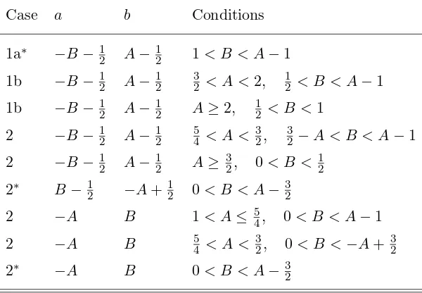
Table 1. Superpotential parameters for rationally-extended Scarf I potentials in the quadratic case.
Case a b Conditions
1a∗ −B−1
2 A−12 1< B < A−1
1b −B−12 A−12 32 < A <2, 12 < B < A−1
1b −B−12 A−21 A≥2, 12 < B <1
2 −B−1
2 A−12 54 < A < 32, 32 −A < B < A−1
2 −B−1
2 A−12 A≥ 32, 0< B < 12
2∗ B−1
2 −A+12 0< B < A−32
2 −A B 1< A≤ 54, 0< B < A−1
2 −A B 54 < A < 23, 0< B <−A+32
2∗ −A B 0< B < A−3 2
range for at least one of the parametersA,B. For simplicity’s sake, they will not be considered any further.
For the selected cases, the two partner potentials can be written as
V(+)(x) =VA′,B′(x), V(−)(x) =VA,B(x) +
N1(x) D(x) +
N2(x)
D2(x), (3.6)
where
A′ =A, B′ =B+ 1,
N1(x) =−4[(2A−1)(2B−1)(2B−2) sinx+ 2(2A−1)2−(2B−2)2(2B+ 1)], N2(x) =−8(2B−2)(2A−2B+ 1)(2A+ 2B−3)
×[2(2A−1)(2B−1) sinx−(2A−1)2−2B(2B−2)],
D(x) = (2B−1)[(2B−2) sinx−(2A−1)]2−(2A−2B+ 1)(2A+ 2B−3) (3.7)
for case I,
A′ =A, B′ =B−1,
N1(x) =−4[(2A−1)(2B+ 1)(2B+ 2) sinx−2(2A−1)2−(2B+ 2)2(2B−1)], N2(x) = 8(2B+ 2)(2A−2B−3)(2A+ 2B+ 1)
×[2(2A−1)(2B+ 1) sinx−(2A−1)2−2B(2B+ 2)],
D(x) = (2B+ 1)[(2B+ 2) sinx−(2A−1)]2+ (2A−2B−3)(2A+ 2B+ 1) (3.8)
for case II, and
A′ =A+ 1, B′ =B,
N1(x) =−8[B(2A−2)(2A−3) sinx−A(2A−3)2+ 4B2], N2(x) = 8(2A−3)(2A−2B−3)(2A+ 2B−3)
×[4B(2A−2) sinx−4B2−(2A−1)(2A−3)],
for case III. Correspondingly,
from which it follows that cases I and II are characterized by strict isospectrality (case ii of SUSYQM), whereas in case III, φ−1(x), which turns out to be normalizable on −π
2,π2
and to vanish at both end points, is the ground-state wavefunction of V(−)(x) with energy eigenvalue
E0(−)=E0(A+1,B)−3(2A−1) = (A−2)2 (caseiiiof SUSYQM).
We conclude that for Scarf I potential, the quadratic case leads to rather similar results to those obtained for the radial oscillator, the form of the rationally-extended potential becoming sensitive to the type of reparametrization made for the starting conventional one.
3.2 Determination of wavefunctions
The procedure used here to determine the wavefunctions of the rationally-extended Scarf I potentials being the same as that introduced in Section 2.2, we will only state the results.
3.2.1 Linear case
The action of this first-order differential operator on the Jacobi polynomial Pν(α−1,β+1)(z) can be easily proved to be given by
where
Nν(−)=
B
2A−2
(2A+ 2ν)ν! Γ(2A+ν)
A−B+ν+12
A+B+ν+12
Γ A−B+ν−12
Γ A+B+ν−12 !1/2
. (3.13)
Had we started from the Scarf I potentialVA,B−1(x), we would have been led to computing
the action of
ˆ
O2(α,β)≡[β+α−(β−α)z]
(1−z) d
dz −(α+ 1)
+ (β−α)(1−z)
on Pν(α+1,β−1)(z). Since ˆO1(α,β) is changed into −Oˆ2(α,β) under the permutation of α with β, combined with the transformation z → −z, we would have obtained the same results (3.12) and (3.13) as before, up to some irrelevant overall sign.
ˆ
Pν(α,β+1)(z), ν = 0,1,2, . . ., form the second complete orthogonal set of polynomials with re-spect to some positive-definite measure that was constructed in [28,29] by starting with some linear polynomial. As recalled in Appendix B, these X1-Jacobi polynomials can be expressed
as linear combinations of three classical Jacobi ones with constant coefficients. They are nor-malized in such a way that their highest-degree term is−2−ν−1 2ν+α+β
ν
zν+1 (as compared with 2−ν 2ν+α+β
ν
zν for Pν(α,β)(z)). In the same appendix, two special cases of well-behaved poten-tials V(−)(x) outside the allowed range 0 < B < A−1 of parameter values are considered in connection with two so far unknown limiting properties of ˆPν(+1α,β)(z).
Observe that the first occurrence of the rationally-extended Scarf I potential (3.5) and of the exceptional X1-Jacobi polynomials in quantum mechanics can be traced back to [34], where
it was also demonstrated that such a potential is shape invariant with a partner given by
VA+1,B,ext(x).
We now plan to generalize ˆPν(α,β+1)(z) to the more sophisticated extended potentials introduced in Section 3.1.2.
3.2.2 Quadratic case
Let us start by considering the rationally-extended potential corresponding to case I and defined in equations (3.6) and (3.7). In calculating its wavefunctions, we arrive at the first-order differential operator
˜
O1(α,β)≡ D(z)
(1 +z) d
dz +β+ 1
−(1 +z) ˙D(z), (3.14)
where α=A−B−12, β=A+B−12, and D(z) amounts to the functionD(x) re-expressed in terms ofz= sinx, while ˙D(z) denotes its derivative with respect toz, i.e.,
D(z) = (β−α−2)[(β−α−1)(β−α−2)z2−2(β−α−1)(β+α)z+ (β+α)2+β−α−2],
˙
D(z) = 2(β−α−1)(β−α−2)[(β−α−2)z−(β+α)].
Such an operator leads to a new family of (ν+ 2)th-degree Jacobi-type polynomials ˜P1(,να,β+2)(z), defined by
˜
O1(α,β)Pν(α−1,β+1)(z) = 4(β−α−1)(β−α−2)2(ν+β−1) ˜P1(,να,β+2)(z)
= β−α−2 2ν+β+α
nh
(β−α−1)(β−α−2)(2ν+β+α)(ν+β−1)z2
+ (ν+β+ 1)(2ν+β+α)[(β+α)2+β−α−2] + 2(β−α−1)(β+α)2iPν(α,β)(z)
For the case II potential given in equations (3.6) and (3.8), it turns out that the first-order differential operator ˜O(2α,β), appearing in the calculation of its wavefunctions, satisfies the same type of symmetry relation with ˜O1(α,β) of equation (3.14) as that connecting ˆO
mutingα withβ and changingzinto−z. As a result, no new family of Jacobi-type polynomials arises for such a potential, its wavefunctions being expressed as
ψ(−)ν (x) = (−1)νNν(−)
in terms of the (ν+ 2)th-degree Jacobi-type polynomials defined in (3.15).
Finally, for the case III potential defined in (3.6) and (3.9), the counterpart of (3.14) reads
+ (β+α+ 2ν)(β+α+ 2ν+ 1)(β+α+ 2ν+ 2)z2] ˙D(z)iPν(α,β)(z)
+ 2(α+ν)(β+ν)h(β+α+ν+ 2)(β+α+ 2ν+ 2)D(z)
−[(β−α) + (β+α+ 2ν+ 2)z] ˙D(z)iPν(α,β−1)(z)o.
The extended-potential excited-state wavefunctions can be written as
ψ(−)ν+1(x) =Nν(−)+1
(1−sinx)12(A−B)(1 + sinx) 1 2(A+B)
D(x) P˜
(A−B−12,A+B− 1 2)
3,ν+3 (sinx),
Nν(−)+1=
(A−1)(2A−3)2 2A−3
(2A+ν−1)(2A+ 2ν+ 2)ν! Γ(2A+ν+ 2) (ν+ 3)Γ A−B+ν+32
Γ A+B+ν+32 !1/2
.
It is obvious that the two families of Jacobi-type polynomials that we have just introduced are of a different nature. From physical considerations, the first set of polynomials ˜P1(,να,β+2)(z), whose lowest-degree one is quadratic in z (see Appendix C), is a good candidate for the still unknown complete, orthogonal family of X2-Jacobi polynomials. By analogy with classical and X1-Jacobi polynomials, ˜P1(α,β,ν+2)(z) has been normalized in such a way that its highest-degree term
is 2−ν−2 2ν+α+β ν
zν+2. By contrast, the other family ˜P(α,β)
3,ν+3(z), starting with a cubic polynomial,
cannot be complete. Note that the highest-degree term is now given by−2−ν−3 2ν+α+β+2 ν
zν+3.
Let us emphasize that for Jacobi-type polynomials, no splitting similar to that observed when going from ˆL(να+1) (z) to ˜L1(α,ν)+2(z) and ˜L(2α,ν)+2(z) has been encountered.
Finally, in cases I and II, the polynomial ˜P(A−B− 1 2,A+B−
1 2)
1,2 (sinx) (or its counterpart) can be
inserted in the extended potential ground-state wavefunction ψ0(−)(x) to prove that the corre-sponding potential VA,B,ext(x) is shape invariant, its partner being given by VA+1,B,ext(x) (see
AppendixD). This again generalizes a result of [34] to the quadratic case.
4
Final comments
In the present paper, we have generated new exactly solvable rationally-extended radial oscillator and Scarf I potentials and we have constructed their bound-state wavefunctions. This has been made possible by generalizing a constructive SUSYQM method recently proposed in [27] and based on some reparametrization of the conventional superpotential, together with the addition of a rational term expressed in terms of a polynomialg(z), wherezis some appropriately chosen function of x. The cases of linear and quadratic polynomials have been considered here.
In the linear case, there appears a single rationally-extended potential, but it can be obtained by starting from an isospectral conventional potential with two distinct sets of reparametrized couplings. In contrast, the quadratic case leads to a variety of rationally-extended potentials, each of them being the partner of a single reparametrized conventional potential. Some potential pairs turn out to be isospectral, while in others, the rational potential has an extra bound state below the conventional potential spectrum.
All rationally-extended potentials belonging to isospectral pairs have been demonstrated to be shape invariant as their conventional counterparts.
Furthermore, by applying our SUSYQM approach, we have explicitly shown that the (ν +1)th-degree polynomials (ν = 0,1,2, . . .) occurring in the bound-state wavefunctions of the extended potentials corresponding to the linear case are the X1-Laguerre or X1-Jacobi polynomials that
them, we have identified two different kinds of (ν + 2)th-degree Laguerre-type polynomials and a single one of (ν+ 2)th-degree Jacobi-type polynomials, which are candidates for the still unknownX2-Laguerre and X2-Jacobi exceptional polynomials, respectively.
Two interesting properties, dealt with in [27], have not been considered here, but are worth mentioning. To begin with, our first-order SUSY transformation may be combined with another one relating conventional potentials with different parameters to produce a reducible second-order SUSY transformation connecting conventional and extended potentials with the same parameters. In the linear case, this results in a second-order transformation admitting two distinct factorizations.
The other point has to do with the possibility of discarding the restriction to real potentials, which has been implicitly made here. Considering alsoPT-symmetric complex potentials indeed facilitates reconciling our approach to the requirement that the rationally-extended potentials be singularity free, hence generating so far unknown complex potentials with a real spectrum. The generalization of the present work along these lines is therefore an interesting topic for future investigation.
When the present work was in its final stage, there appeared two interesting preprints, whose subjects are related to those considered here. In the first one [36], the existence of distinct factorizations of second-order SUSY transformations into products of two first-order ones, observed for the rationally-extended generalized P¨oschl–Teller potential of [27] and which would also be obtained here in the linear case, is discussed in the framework of type A 2-fold SUSY [22]. Necessary and sufficient conditions for such a situation to occur are derived and some relations to second-order parasupersymmetry and generalized 2-fold superalgebras are noted.
In the second work [37], three infinite families of shape-invariant, rationally-extended radial oscillator, trigonometric and hyperbolic P¨oschl–Teller potentials are presented. They are ob-tained by deforming the corresponding conventional potentials in terms of their degreeℓ polyno-mial eigenfunctions and their bound-state wavefunctions are expressed in terms of Laguerre-type or Jacobi-type polynomials. In the radial oscillator and trigonometric P¨oschl–Teller cases, the first member of the infinite family, corresponding to ℓ= 1, is shown to coincide with one of the potentials introduced in [34] and re-obtained here in the linear case for the radial oscillator and Scarf I, respectively.
The general expressions provided both for the potentials and the polynomials in [37] enable us to pursue the comparison with the results of [27] and those derived here. To start with, it can be easily seen that the first member (with ℓ = 1) of the third family (hyperbolic P¨oschl– Teller) actually corresponds via some changes of variable and of parameters (x → x/2, g → B −A−1, h → B +A+ 1) to the extended generalized P¨oschl–Teller potential constructed in [27]. Furthermore, the results corresponding to the second member (withℓ= 2) of the first two families agree with those of the present paper associated with the quadratic case and referred to as case I extended radial oscillator and case II extended Scarf I, respectively. It should be stressed that no case II extended radial oscillator (with its corresponding Laguerre-type polynomials) is found there. Whether the existence of such an alternative branch of potentials and polynomials, demonstrated in the quadratic case in the present paper, could be generalized to higher-degree polynomialsg(z) would be an interesting topic for future investigation.
A
Examples of Laguerre-type polynomials
In this appendix, we list the first few ˜L(1α,ν)+2, ˜L(2α,ν)+2, and ˜L(3α,ν)+3Laguerre-type polynomials and, for comparison’s sake, also the corresponding classical and X1-Laguerre polynomials.
Laguerre polynomials
L(1α)(z) =−z+α+ 1,
L(2α)(z) = 12[z2−2(α+ 2)z+ (α+ 2)(α+ 1)].
X1-Laguerre polynomials
ˆ
L(1α)(z) =−z−α−1,
ˆ
L(2α)(z) =z2−α(α+ 2),
ˆ
L(3α)(z) = 12[−z3+ (α+ 3)z2+α(α+ 3)z−α(α+ 1)(α+ 3)].
New Laguerre-type polynomials
˜
L(1α,2)(z) =z2+ 2(α+ 2)z+ (α+ 2)(α+ 1),
˜
L(1α,3)(z) =−z3−(α+ 3)z2+α(α+ 3)z+α(α+ 1)(α+ 3),
˜
L(1α,4)(z) = 12[z4−2(α+ 1)(α+ 4)z2+α(α+ 1)2(α+ 4)],
˜
L(2α,2)(z) =z2+ 2αz+α(α+ 1),
˜
L(2α,3)(z) =−z3−(α−1)z2+ (α+ 2)(α−1)z+ (α+ 2)(α+ 1)(α−1),
˜
L(2α,4)(z) = 12[z4−4z3−2(α+ 3)(α−1)z2+ (α+ 3)(α+ 2)α(α−1)],
˜
L(3α,3)(z) = 13[−z3+ 3(α−1)z2−3α(α−1)z+ (α+ 1)α(α−1)],
˜
L(3α,4)(z) = 14[z4−4αz3+ 2(α−1)(3α+ 4)z2−4(α+ 2)α(α−1)z
+ (α+ 2)(α+ 1)α(α−1)],
˜
L3(α,5)(z) = 101[−z5+ 5(α+ 1)z4−10(α2+ 2α−1)z3+ 10(α+ 3)(α+ 1)(α−1)z2
−5(α+ 3)(α+ 2)α(α−1)z+ (α+ 3)(α+ 2)(α+ 1)α(α−1)].
B
Limiting cases of extended Scarf I potentials
and of
X
1-Jacobi polynomials
The purpose of this appendix is to review two cases where although the parameter B in the rationally-extended Scarf I potential (3.5) takes a value outside the allowed range 0< B < A−1, the potential remains physically acceptable and reduces to some known conventional potential. As a result, there exists a limiting relation between the wavefunctions of the former, given in equations (3.12) and (3.13), and those of the latter, expressed in terms of some classical polynomials. The corresponding properties of the X1-Jacobi polynomials will be demonstrated
by starting from their known ones, proved in [29].
If we setB = 0 in equation (3.5), the sum of the two rational terms vanishes and we get the
B → 0 limit of the Scarf I potential, which is the one-parameter trigonometric P¨oschl–Teller potential VA,0(x) = A(A−1) sec2x. Its energy spectrum is given by equation (3.1) and the
corresponding wavefunctions can be expressed in terms of Gegenbauer polynomials as [38]
ψ(νA,0)(x) = ¯Nν(A)(cosx)ACν(A)(sinx),
where
¯
Nν(A) =
Γ(A)Γ(2A)ν! (A+ν)
√
πΓ A+ 12
Γ(2A+ν)
!1/2
Comparison with equations (3.12) and (3.13) leads to the relation
The direct proof of equation (B.1) is based on the expansion of X1-Jacobi polynomials as
linear combinations of three classical Jacobi ones,
ˆ
On the other hand, we observe that although the Scarf I potentialVA,B(x) is not defined for
B =A−1
2 orA=B+12, the same is not true for its extensionVA,B,ext(x), given in equation (3.5).
The latter is indeed equivalent to the well-behaved conventional Scarf I potential VA+1,A−3 2(x)
with energy spectrum Eν(A+1) = (A+ν+ 1)2,ν = 0,1,2, . . ., and wavefunctionsψ(
A+1,A−3 2) ν (x), obtainable from equation (3.2). For the same parameter values, we get from equation (3.12)
lim B→A−12
ψ(−)0 (x)∝(1−sinx)−34(1 + sinx)A− 1
4[2A+ 1−(2A−1) sinx],
which does not vanish forx→ π2, hence is not physically acceptable. This explains the absence of an eigenvalue A2 in the energy spectrum. The presence of the remaining eigenvalues, corre-sponding to ν = 1,2, . . ., in (3.1) hints at a limiting relation between ˆP(A−B−
On using equations (22.7.18) and (22.7.15) of [32], it is straightforward to transform the latter into
C
Examples of Jacobi-type polynomials
In this appendix, we list the first few ˜P1(,να,β+2) and ˜P3(,να,β+3) Jacobi-type polynomials and, for com-parison’s sake, also the corresponding classical and X1-Jacobi polynomials.
Jacobi polynomials
P0(α,β)(z) = 1,
P1(α,β)(z),= 12[(β+α+ 2)z−(β−α)].
X1-Jacobi polynomials
ˆ
P1(α,β)(z) = 1
2(β−α)[−(β−α)z+β+α+ 2],
ˆ
P2(α,β)(z) = 1
4(β−α){−(β−α)(β+α+ 2)z
2+ [(β−α)2+ (β+α)(β+α+ 4)]z
−(β−α)(β+α+ 2)}.
New Jacobi-type polynomials
˜
P1(,α,β2 )(z) = 1
4(β−α−1)(β−α−2)[(β−α−1)(β−α−2)z
2
−2(β−α−1)(β+α+ 2)z+ (β+α+ 2)2+β−α−2],
˜
P1(,α,β3 )(z) = 1
8(β−α−1)(β−α−2){(β−α−1)(β−α−2)(β+α+ 2)z
3
−(β−α−1)[(β−α)(β−α−2) + 2(β+α)(β+α+ 4)]z2
+ (β+α+ 2)[(β−α−2)(2β−2α+ 3) + (β+α)(β+α+ 4)]z
−(β−α)(β+α+ 2)2−(β−α−4)(β−α+ 2)},
˜
P3(,α,β3 )(z) = 1
8(β+α)(β+α−1)(β+α−2){−(β+α)(β+α−1)(β+α−2)z
3
+ 3(β+α)(β+α−1)(β−α)z2−3(β+α)[(β−α)2+β+α−2]z
+ (β−α)[(β−α)2+ 3β+ 3α−4]},
˜
P3(,α,β4 )(z) = 1
16(β+α−1)(β+α−2)(β+α+ 1)
× {−(β+α−2)(β+α−1)(β+α+ 1)(β+α+ 4)z4
+ 4(β−α)(β+α−1)(β+α+ 1)(β+α+ 2)z3
−2(β+α+ 1)[(β−α)2(3β+ 3α+ 2) + (β+α−2)(β+α+ 4)]z2
+ 4(β−α)(β+α+ 1)[(β−α)2+β+α−2]z
−(β−α)4−2(β−α)2(β+α−4) + (β+α−2)(β+α+ 4)}.
D
Shape invariance of rationally-extended potentials
In such a picture corresponding to case i of SUSYQM, the rationally-extended poten-tial is considered as the starting potenpoten-tial ˜V(+)(x) and its partner is determined from
equa-tion (2.6) as ˜V(−)(x) = ˜V(+)(x) + 2 ˜W′(x), where the superpotential is now given by ˜W(x) =
−d[ln ˜ψ0(+)(x)]/dx, with ˜ψ(+)0 (x) =ψ0(−)(x).
On using the expressions found forψ(−)0 (x) in Section 2.2.2 and the results of Appendix A, it is straightforward to show that for case I and II extended radial oscillator potentials,
˜
W(x) = ˜W1(x) + ˜W2(x), W˜1(x) =
1 2ωx−
l+ 1
x ,
and
˜
W2(x) = 4ωx
ωx2+ 2l+ 3
(ωx2+ 2l+ 3)2−2(2l+ 3)−
ωx2+ 2l+ 5
(ωx2+ 2l+ 5)2−2(2l+ 5)
(case I),
˜
W2(x) = 4ωx
ωx2+ 2l−1
(ωx2+ 2l−1)2+ 2(2l−1)−
ωx2+ 2l+ 1 (ωx2+ 2l+ 1)2+ 2(2l+ 1)
(case II),
from which it directly follows that
2 ˜W′(x) =−Vl,ext(x) +Vl+1,ext(x) +ω.
Hence, in such cases, the partner ofVl,ext(x) isVl+1,ext(x) +ω, which proves the shape invariance
of the former.
Similarly, from Section3.2.2 and Appendix C, we obtain for case I and II extended Scarf I potentials,
˜
W(x) = ˜W1(x) + ˜W2(x), W˜1(x) =Atanx−Bsecx,
and
˜
W2(x) = 2(2B−1)(2B−2) cosx
×
(2B−2) sinx−(2A−1)
DA,B(x) −
(2B−2) sinx−(2A+ 1)
DA+1,B(x)
(case I),
˜
W2(x) = 2(2B+ 1)(2B+ 2) cosx
×
(2B+ 2) sinx−(2A−1)
DA,B(x) −
(2B+ 2) sinx−(2A+ 1)
DA+1,B(x)
(case II),
where DA,B(x) denotes the denominator functionD(x) of equations (3.7) and (3.8), associated with some specified parameters A,B. Since
2 ˜W′(x) =−VA,B,ext(x) +VA+1,B,ext(x),
the partner ofVA,B,ext(x) is VA+1,B,ext(x), thus completing the proof.
Acknowledgements
References
[1] Bargmann V., On the connection between phase shifts and scattering potential, Rev. Modern Phys. 21
(1949), 488–493.
[2] Sukumar C.V., Supersymmetric quantum mechanics of one-dimensional systems, J. Phys. A: Math. Gen.
18(1985), 2917–2936.
[3] Cooper F., Khare A., Sukhatme U., Supersymmetry and quantum mechanics,Phys. Rep.251(1995), 267–
385,hep-th/9405029.
[4] Junker G., Supersymmetric methods in quantum and statistical physics,Text and Monographs in Physics, Springer-Verlag, Berlin, 1996.
[5] Bagchi B., Supersymmetry in quantum and classical mechanics, Chapman &Hall/CRC Monographs and Surveys in Pure and Applied Mathematics, Vol. 116, Chapman & Hall/CRC, Boca Raton, FL, 2000. [6] Mielnik B., Rosas-Ortiz O., Factorization: little or great algorithm?, J. Phys. A: Math. Gen. 37(2004),
10007–10035.
[7] Infeld L., Hull T.E., The factorization method,Rev. Modern Phys.23(1951), 21–68.
[8] Fatveev V.V., Salle M.A., Darboux transformations and solitons, Springer Series in Nonlinear Dynamics, Springer, New York, 1991.
[9] Mielnik B., Factorization method and new potentials with the oscillator spectrum,J. Math. Phys.25(1984),
3387–3389.
[10] Mitra A., Roy P.K., Lahiri A., Bagchi B., Nonuniqueness of the factorization scheme in quantum mechanics,
Internat. J. Theoret. Phys.28(1989), 911–916.
[11] Junker G., Roy P., Conditionally exactly solvable problems and non-linear algebras, Phys. Lett. A 232
(1997), 155–161.
[12] Bagchi B., Quesne C., Zero-energy states for a class of quasi-exactly solvable rational potentials, Phys. Lett. A230(1997), 1–6,quant-ph/9703037.
[13] Blecua P., Boya L.J., Segui A., New solvable quantum-mechanical potentials by iteration of the freeV = 0 potential,Nuovo Cimento Soc. Ital. Fis. B118(2003), 535–546,quant-ph/0311139.
[14] G´omez-Ullate D., Kamran N., Milson R., The Darboux transformation and algebraic deformations of shape-invariant potentials,J. Phys. A: Math. Gen.37(2004), 1789–1804,quant-ph/0308062.
[15] G´omez-Ullate D., Kamran N., Milson R., Supersymmetry and algebraic Darboux transformations,
J. Phys. A: Math. Gen.37(2004), 10065–10078.
[16] Cari˜nena J.F., Perelomov A.M., Ra˜nada M.F., Santander M., A quantum exactly solvable nonlinear oscil-lator related to the isotonic osciloscil-lator,J. Phys. A: Math. Theor.41(2008), 10 pages,arXiv:0711.4899.
[17] Andrianov A.A., Ioffe M.V., Cannata F., Dedonder J.-P., Second order derivative supersymmetry,q defor-mations and the scattering problem,Internat. J. Modern Phys. A10(1995), 2683–2702,hep-th/9404061.
[18] Andrianov A.A., Ioffe M.V., Nishnianidze D.N., Polynomial supersymmetry and dynamical symmetries in quantum mechanics,Theoret. and Math. Phys.104(1995), 1129–1140.
[19] Andrianov A.A., Ioffe M.V., Nishnianidze D.N., Polynomial SUSY in quantum mechanics and second deriva-tive Darboux transformations,Phys. Lett. A201(1995), 103–110,hep-th/9404120.
[20] Samsonov B.F., New features in supersymmetry breakdown in quantum mechanics,Modern Phys. Lett. A
11(1996), 1563–1567,quant-ph/9611012.
[21] Bagchi B., Ganguly A., Bhaumik D., Mitra A., Higher derivative supersymmetry, a modified Crum–Darboux transformation and coherent state,Modern Phys. Lett. A14(1999), 27–34.
[22] Aoyama H., Sato M., Tanaka T.,N-fold supersymmetry in quantum mechanics: general formalism,Nuclear Phys. B619(2001), 105–127,quant-ph/0106037.
[23] Fern´andez C. D.J., Fern´andez-Garc´ıa N., Higher-order supersymmetric quantum mechanics, Latin-American School of Physics – XXXV ELAF,AIP Conf. Proc., Vol. 744, Amer. Inst. Phys., Melville, NY, 2005, 236–273,
quant-ph/0502098.
[24] Contreras-Astorga A., Fern´andez C. D.J., Supersymmetric partners of the trigonometric P¨oschl–Teller po-tentials,J. Phys. A: Math. Theor.41(2008), 475303, 18 pages,arXiv:0809.8760.
[25] Duistermaat J.J., Gr¨unbaum F.A., Differential equations in the spectral parameter, Comm. Math. Phys.
[26] Erd´elyi A., Magnus W., Oberhettinger F., Tricomi F.G., Higher transcendental functions, Mc-Graw Hill, New York, 1953.
[27] Bagchi B., Quesne C., Roychoudhury R., Isospectrality of conventional and new extended potentials, second-order supersymmetry and role ofPT symmetry,Pramana J. Phys.73(2009), 337–347,arXiv:0812.1488.
[28] G´omez-Ullate D., Kamran N., Milson R., An extension of Bochner’s problem: exceptional invariant sub-spaces,arXiv:0805.3376.
[29] G´omez-Ullate D., Kamran N., Milson R., An extended class of orthogonal polynomials defined by a Sturm– Liouville problem,J. Math. Anal. Appl.359(2009), 352–367,arXiv:0807.3939.
[30] Moshinsky M., Smirnov Yu.F., The harmonic oscillator in modern physics, Harwood, Amsterdam, 1996.
[31] Gendenshtein L.E., Derivation of exact spectra of the Schr¨odinger equation by means of supersymmetry,
JETP Lett.38(1983), 356–359.
[32] Abramowitz M., Stegun I.A., Handbook of mathematical functions with formulas, graphs, and mathematical tables,National Bureau of Standards Applied Mathematics Series, Vol. 55, Washington, D.C., 1964. [33] Bochner S., ¨Uber Sturm-Liouvillsche Polynomsysteme,Math. Z.29(1929), 730–736.
[34] Quesne C., Exceptional orthogonal polynomials, exactly solvable potentials and supersymmetry,J. Phys. A: Math. Theor.41(2008), 392001, 6 pages,arXiv:0807.4087.
[35] Bhattacharjie A., Sudarshan E.C.G., A class of solvable potentials,Nuovo Cimento25(1962), 864–879.
[36] Bagchi B., Tanaka T., Existence of different intermediate Hamiltonians in type AN-fold supersymmetry,
arXiv:0905.4330.
[37] Odake S., Sasaki R., Infinitely many shape invariant potentials and new orthogonal polynomials,
arXiv:0906.0142.
[38] Quesne C., Comment: “Application of nonlinear deformation algebra to a physical system with P¨oschl– Teller potential” [Chen J.-L., Liu Y., Ge M.-L.,J. Phys. A: Math. Gen.31(1998), 6473–6481],J. Phys. A: