Directory UMM :Journals:Journal of Health Economics:Vol19.Issue1.Jan2000:

(1)

www.elsevier.nlrlocatereconbase

Did the Medicaid expansions for children

displace private insurance? An analysis using

the SIPP

Linda J. Blumberg

a,)

_{, Lisa Dubay}

a

_{, Stephen A. Norton}

b

a

The Urban Institute, 2100 M Street, NW, Washington, DC 20037, USA

b

New Hampshire Department of Health and Human SerÕices, USA

Abstract

Using data from the 1990 panel of the Survey of Income and Program Participation ŽSIPP , we address the question: Did the Medicaid expansions for children cause declines in. private coverage? We use a multivariate approach that attributes a displacement effect to declines in private coverage for children targeted by the Medicaid expansions exceeding declines for a comparison group of older low-income children. We find that 23% of the movement from private coverage to Medicaid due to the expansions was attributable to displacement. There is no evidence of displacement among those starting uninsured, leading to an overall displacement effect of 4%.q_{2000 Elsevier Science B.V. All rights reserved.}

Keywords: Medicaid; Private health insurance; Crowd-out

1. Introduction

Until the late 1980s, Medicaid eligibility for children had been limited to children in welfare families and later extended to children in two-parent families with incomes below welfare eligibility thresholds. In response to declining health status indicators for low-income children and growing disparities in health status

Ž

and utilization between the insured and the uninsured Rosenbach, 1985; Kasper,

.

1987; Leftkowitz and Short, 1989; Short and Leftkowitz, 1991 , beginning in

) _{Corresponding} _author. _Tel.: _q_{1-202-261-5769;} _fax: _q_{1-202-223-1149;} _E-mail:

lblumber@ui.urban.org

Ž .

(2)

1988, Congress permitted and eventually mandated states to provide Medicaid coverage for children in higher-income families. As of April 1990, coverage became mandatory for children up to age 6 in families with incomes up to 133% of the federal poverty level. As of July 1991, coverage became mandatory for children born after September 30, 1983 with family incomes up to 100% of

Ž .

poverty. Federal legislation also gave states the option starting in 1988 of covering infants with family incomes up to 185% of poverty. These expansions were intended to reduce the number of uninsured children, improve children’s access to health care, and, thus, improve their health.

Between 1988 and 1993, the number of children receiving Medicaid-covered services grew by 53%.1 _{Over the same period, however, employer-sponsored}

Ž .

insurance coverage declined Peat Marwick, 1994; Holahan et al., 1995 , and the

Ž .

number of uninsured children grew Dubay and Kenney, 1996 . This combination of trends has led some to question whether the Medicaid expansions for children

Ž

and pregnant women ‘‘crowded-out’’ employer-sponsored coverage Cutler and Gruber, 1996a,b; Dubay and Kenney, 1996, 1997; Yazici and Kaestner,

forthcom-.

ing rather than expanded coverage for those who would have continued to be uninsured in its absence.

Crowd-out is a term that covers two potential unintended consequences of the

Ž .

Medicaid eligibility expansion: 1 persons with private coverage drop it in order

Ž .

to take advantage of the public subsidy being offered; and 2 some who are

Ž

uninsured enroll in Medicaid rather than obtain private coverage as they would

.

have under the more stringent Medicaid eligibility conditions . A related possibil-ity is that employers use the availabilpossibil-ity of publicly sponsored plans to discontinue

Žor not begin offering group coverage to their employees. Crowd-out can have.

two major policy implications. The substitution of Medicaid for private coverage may lead to fewer improvements in access to care and health status because the change from being uninsured to insured is more limited than expected.2_Crowd-out

may also lead to greater increases in Medicaid expenditures than expected as

1

Unpublished Urban Institute tabulations of HCFA Form 2082 data.

2 _Ž _.

(3)

individuals who previously had private insurance drop it to enroll in the subsidized public program. However, providing Medicaid coverage, an income transfer to the low-income population, may be considered desirable regardless of previous insur-ance status.

The essential policy question is: Did the Medicaid expansions cause the private coverage declines or were the two contemporaneous trends actually independent? This is a difficult question to answer because of the many factors that have to be disentangled to establish causation. In this paper, we use data from the 1990 panel

Ž .

of the Survey of Income and Program Participation SIPP to address this policy question. The SIPP is a nationally representative longitudinal database that allows us to track insurance coverage transitions of specific children over the 32-month period during which the mandated expansions were implemented. We compare health insurance coverage transitions of one group of low-income children affected and another group unaffected by the expansions. Our analysis extends the previous literature by using nationally representative longitudinal data to calculate separate effects for children who were privately insured prior to the mandated increases in Medicaid eligibility thresholds and for children who were uninsured before the mandatory Medicaid expansions. We do not address the issue of whether employ-ers are making decisions to offer insurance coverage to their employees or not. Nor do we assess whether the expansions led some families to remain in the Medicaid program for longer periods before obtaining private coverage than they would have without the expansions. We find that 23% of the movement from private coverage to the Medicaid program as a result of the expansions was due to the displacement of private coverage. We find no evidence that the expansions discouraged families with uninsured children from taking up private coverage.

Section 2 summarizes the literature on the subject of crowd-out. Section 3 presents our methodological approach and Section 4 describes the data used. Section 5 presents our empirical results. Section 6 summarizes our findings and conclusions.

2. Previous literature

(4)

of the expansions, each poses different questions and measures the extent of

3 _Ž

crowd-out in different ways, making it difficult to compare their results. For a

.

full discussion of the relevant literature, see Dubay, 1999.

Ž .

Cutler and Gruber 1996a; b were the first to assess the extent of crowd-out under the Medicaid expansions and used individual level data from the 1987 through 1993 CPS. The work by Cutler and Gruber makes a number of different crowd-out estimates. In contrast to the other studies that use different low-income populations to account for what would have happened in the absence of the expansions, Cutler and Gruber use the experience of non-eligible populations, regardless of income, to control for trends in insurance coverage. Their estimates are identified from cross-state differences in changes in eligibility. For children, they find that between 31 and 41% of the increase in Medicaid coverage, that occurred as a result of the expansion in eligibility, was offset by declines in private coverage resulting from the expansions. Accounting for conditional coverage and spillover effects,4 Cutler and Gruber estimate that for every two people who enrolled in Medicaid as a result of the expansions, one person dropped his private insurance, a 50% effect. However, they note that ‘‘80% of the increase in

w x

Medicaid as a result of the expansions , or 2.8 million people, was from those who were formerly uninsured’’ an alternatively measured crowd-out rate of 20%

Ž_{Cutler and Gruber, 1996a,b . The difference in their two estimates is due to the}.

fact that not everyone they identified as dropping private insurance as a result of the expansions was eligible for Medicaid; many were non-eligible family members

Ž .

of eligible individuals i.e., a spillover effect .

Ž .

Dubay and Kenney 1996; 1997 also used the CPS to examine the extent of crowd-out that occurred with the Medicaid expansions. Dubay and Kenney limit their analysis to low-income young children and pregnant women and use low-in-come men to control for the secular trend in insurance coverage. They limit their sample in this way on the grounds that the expansions affected only a small portion of the entire population, and the secular declines in employer-sponsored insurance that were occurring for the group targeted by the expansions were likely to have been dissimilar to the declines for the whole population. They find that overall 14% of the total increase in Medicaid enrollment of pregnant women, and 17% of the total increase in enrollment of young children that occurred over the expansion period were attributable to crowd-out.

3 _Ž _.

Shore-Sheppard 1997 has also looked at this issue.

4

(5)

Ž .

Yazici and Kaestner forthcoming use the 1988 and 1992 waves of the NLSY, a longitudinal database, and analyze low-income children who were under age 9. They use two groups of low-income children who were never eligible for

Ž

Medicaid to account for the secular trend in coverage those whose families had a

.

loss of income and those whose families had no loss of income . Yazici and Kaestner make separate crowd-out estimates for children who were eligible for Medicaid in 1988, and two groups of children who became eligible for Medicaid

Ž .

by 1992 those whose families did and did not experience a loss of income . Similar to Dubay and Kenney, Yazici and Kaestner estimate that overall 19% of the increase in Medicaid coverage that occurred over this period for their cohort of low-income young children was attributable to crowd-out.

Ž .

Finally, Thorpe and Florence 1998 take a different approach to measuring crowd-out using data from the 1989 through 1994 waves of the NLSY. They define as crowd-out the movement of a child into Medicaid when hisrher parent

Ž

has private coverage i.e., they use the children’s parents as a control for what

.

would have happened in the absence of the expansions . They find that for children living in poverty who moved into the Medicaid program from private insurance, between 1 and 14% had parents who maintained private coverage, depending on the year being examined. For children with incomes above poverty, this percentage ranged from 15 to 20%. When all entrants into the Medicaid program with incomes below 200% of poverty are considered, i.e., those entering from uninsurance and from private coverage, they estimate that 16% of all children who entered the Medicaid program in 1990 and 1994 did so as the result of the crowding-out of private coverage.

Our analysis extends the previous literature by examining actual insurance coverage transitions among children affected and unaffected by the expansions and using multivariate analysis to estimate the share of ‘‘expansion-related’’ move-ment into the Medicaid program that was due to crowd-out. We estimate separate crowd-out effects for children who had private coverage prior to the expansions, for children who were uninsured prior to the expansions, and an overall effect. We use the experience of a group of slightly older children who have similar family incomes to those children targeted by the expansions to control for other changes occurring over the expansion period.

3. Methods

We assess whether and to what extent the Medicaid expansions for children displaced private coverage by examining the health insurance coverage of

low-in-Ž

come children at the first interview of the 1990 SIPP panel prior to the mandated

. Ž .

(6)

children affected by the expansions in eligibility with changes for a comparison group of children who were unaffected by the expansions. Applying multivariate regression models to this quasi-experimental design, we produce three estimates that together indicate the extent of crowd-out overall and among the two compo-nent populations: the percentage of the movement from priÕate coÕerage into the

Medicaid program due to crowd-out; the percentage of the movement from

Ž

uninsurance into the Medicaid program due to crowd-out i.e., families choosing

.

not to obtain private coverage ; and the overall percentage of the movement into the Medicaid program due to crowd-out.

3.1. Analytic approach

Ž

Even with longitudinal data, as noted, determining causation, i.e., whether the

.

Medicaid expansions actually displaced private insurance is complicated. In order to isolate displacement from other factors, we need to disentangle the impacts of the expansions from the impacts of these other factors. Otherwise, we risk

Ž .

overestimating underestimating the extent to which the expansions displaced

Ž .

private insurance by falsely attributing to neglecting to attribute to the expan-sions movement out of private coverage into Medicaid which was actually

Ž .

unrelated related .

Our method of controlling for the impacts of these other factors is to subtract the insurance changes of a comparison group of children from the insurance coverage changes of the target group of children. This difference-in-differences approach only attributes to the expansions any decline in private coverage for the target group that is greater than that for the comparison group. This approach assumes that the impact of any other factor that might affect these patterns, beyond those that we control for explicitly, was the same for the two groups.

The 1990 panel of the SIPP collects information over a 32-month period beginning in the last quarter of 1989. Our target group consists of children born after September 30, 1983 — essentially children under age 7 at the beginning of the panel — with incomes below 185% of poverty at the first interview.5

Depending on family income, some of these children became eligible for Medicaid over the course of the panel as a result of the mandated expansions, while others were eligible through the traditional eligibility routes or optional expansion routes available from the beginning of the panel. The comparison group consists of slightly older children in families with incomes below 185% of poverty at the first interview of the panel. These children were 7 to 11 years old at the first interview. While some of these children were eligible for Medicaid under the traditional eligibility routes at the beginning of the panel, those with higher incomes never became eligible under the expansions due solely to their age. We include children

5

Income as a percentage of poverty is calculated based on income net of standard work deductions

(7)

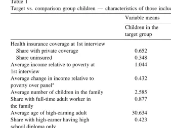
Table 1

Target vs. comparison group children — characteristics of those included in the analysis files Variable means

Children in the Children in the target group comparison group Health insurance coverage at 1st interview

Share with private coverage 0.652 0.639

Share uninsured 0.348 0.361

Average income relative to poverty at 1.044 1.070

1st interview

Average change in income relative to 0.432 0.416

a

poverty over panel

UUU

Average number of children in the family 2.585 2.973

U

Share with full-time adult worker in 0.877 0.910

the family

UUU

Average age of high-earning adult 30.634 35.004

Share with high-earner having high 0.423 0.438

school diploma only

Share with high-earner having some 0.354 0.322

college education

Share with two-parent family 0.770 0.730

Share with white high-earner 0.798 0.768

Share living in the midwest 0.258 0.226

Share living in the south 0.398 0.437

Share living in the west 0.200 0.192

Sample size 1477 1110

a

Expressed as income relative to poverty at last interview minus income relative to poverty at first interview.

U

Difference between target and comparison means is significant at the 0.10 level.

UU

UUU

with incomes up to 185% of poverty rather than limiting the analysis to those with incomes up to 133% of poverty because some of these higher-income children may have become eligible for Medicaid due to declines in family income as a result of the recession.6 We included children in the target and comparison groups based on family income at the first interview.

Table 1 compares initial health insurance coverage and other socio-economic characteristics for the target- and comparison-group children used in our analyses. In most respects, the target group children and the comparison group children appear quite similar. Two statistically significant differences are that the target group children have younger parents on average than their comparison group counterparts and tend to have fewer numbers of children in their families as well.

6

(8)

3.1.1. Estimation strategy

Since the ability of our approach to isolate the effects of the expansions from the effects of other factors depends critically on whether the target group would have had the same health insurance transitions in the absence of the expansions that the comparison group had, we use multivariate methods to hold constant differences in measurable family characteristics potentially associated with the ability of families to obtain and maintain private insurance coverage.7

In order to assess the extent of crowd-out, we estimate three sets of linear probability models.8 _{In the first set, we include only children in the target and}

comparison groups who had private coverage at the first interview of the panel. For these children, we estimate three separate models: the probability of having private coverage at the last interview of the survey; the probability of having Medicaid coverage at the last interview of the survey; and the probability of being uninsured at the last interview of the survey. In the second set, we include only children in the target and comparison groups who were uninsured at the first interview of the survey. For these children, we also estimate three separate models: the probability of being uninsured at the last interview of the survey; the probability of having Medicaid coverage in the last interview of the survey; and the probability of having private coverage at the last interview of the survey. Our third set of models includes all children in the target and comparison groups, regardless of initial insurance status. Again, three models are estimated: the probability of having private coverage in the last interview; the probability of having Medicaid in the last interview; and the probability of being uninsured in the last period.

We model the probability of having a given type of coverage at the last interview of the panel given the type of coverage at the first interview of the panel as:

<

Probability coverage

Ž

i Lsmcoveragei Fsh

.

sa1qa target2 iqa family3 i

qa region ,₄ _i

where: coveragei L is child i’s insurance coverage at the last interview of the survey and m can be private coverage, Medicaid coverage, or uninsurance; coveragei F is child i’s insurance coverage in the first interview of the survey and

h is either private coverage or uninsurance depending upon the set of models;

Ž

target is a binary variable indicating that child i is in the target group as definedi

7

Neither our nor any other analysis can control for unobserved differences associated with differential ability to obtainrmaintain private coverage. This limitation must always be kept in mind in interpreting crowd-out estimates. In our case, e.g., parents may be more likely to go through the Medicaid eligibility determination process for the younger target group children than for the slightly older comparison group children who tend to utilize health care services less frequently.

8

(9)

.

previously ; family is a vector of explanatory variables depicting characteristics ofi

child i’s family; and region is a vector of binary variables indicating the region ofi

the country in which child i resides.

Each independent variable is defined based on information collected at the first panel interview. Family characteristics included in the model are: the number of

Ž

children in the family, the educational attainment of the high-earner less than high

.

school, high school, and at least some college , income as a percentage of poverty, presence of a full-time worker in family, having a two-parent family, and race of the high-earner. Our standard errors are based on a robust estimator of the

Ž .

covariance matrix Huber, 1967; White, 1980 which allows the error terms of observations from children in the same family to be correlated.

In the context of these regressions, the coefficient on the variable ‘target’ in each of these regressions represents the difference between the target and compari-son groups in the probability of being in the initial insurance state at the last

Ž .

interview or of having a different specific type of insurance in the last interview. As mentioned earlier, our approach assumes that any difference between the target and comparison groups, controlling for measurable factors, is due to the expan-sions. Therefore, a lower probability of having private coverage at both the first and last interviews for children in the target group relative to children in the comparison group leads to the conclusion that the expansions did, in fact, displace private insurance coverage. No differences between the target and comparison groups in the probability of having private coverage at these two points lead to the conclusion that there was no crowd-out. Similarly, a lower probability of having private coverage in the last interview, for children in the target group who began the panel uninsured relative to children in the comparison group, leads to the conclusion that there was crowd-out among the uninsured.

If we observe some crowd-out among children who started either with private coverage or who were uninsured, we can then estimate the proportion of the expansion-related movement into Medicaid that was due to private coverage displacement. To calculate the percentage of the expansion-related movement from private coverage into Medicaid that was attributable to crowd-out, we divide the coefficient on ‘target’ in the equation predicting the probability of having private coverage at both the first and last interviews by the coefficient on ‘target’ in the equation predicting the probability of movement from private coverage to Medi-caid coverage. Similarly, we calculate the proportion of expansion-related move-ment into Medicaid from uninsurance that is attributable to crowd-out by dividing the coefficient on ‘target’ in the equation predicting the probability of movement from uninsurance to private coverage by the coefficient on ‘target’ in the equation predicting the probability of moving from uninsurance to Medicaid.9

9

(10)

We also estimate a combined model to assess the overall extent of crowd-out for children moving into the Medicaid program from either private or uninsurance. This model takes a form similar to the equations described above. Specifically, we estimate:

Probability coverage

Ž

i Lsm

.

sb1qb2targetiqb3 uninsurancei

qb4familyiqb5region ,i

where uninsurance is an indicator that child i was uninsured in the first period,i

and the other variables are as noted previously.

3.1.2. Estimation issues

Four estimation issues deserve mention. First, while there are important advan-tages to using longitudinal data such as the SIPP to examine crowd-out rather than cross-sectional data such as the CPS, the relatively small sample size of the SIPP and its complex sampling design reduce our power to detect small differences in outcomes and raise the chance that differences we estimate not to be statistically

Ž .

significant are, in fact, true differences a Type II error . Since the small sample size of the SIPP should not lead to bias, the point estimates of the coefficients, regardless of their statistical significance, can provide insight into the direction and magnitude of any effect.

Second, we are concerned about two types of measurement error that could affect the composition of our target and comparison groups. One is error in family income measurement. Children are included in our sample based on their parent’s reported monthly income at the first interview of the SIPP. If respondents report their income with error, we may include in our target group children who were never affected by the expansions andror exclude children who were affected. To the degree that income is generally underreported on surveys, the likely bias would be to include in our target group individuals who are not actually eligible for the expansions. This type of measurement error would bias our coefficients on ‘target’ downwards. We can net out this bias by calculating crowd-out estimates based on

Ž

the ratio of the coefficients on ‘target’ for two equations Yazici and Kaestner,

.

forthcoming . However, we need to remember that the point estimates on target in each of the equations may be biased downwards.

The other measurement error we are concerned about stems from the fact that children who were eligible for Medicaid under pre-expansion rules are included in both our target and comparison groups. These children may have been affected by outreach efforts and improvements in the eligibility determination process that occurred as part of the expansions in coverage but were not themselves eligible for

Ž .

(11)

interview in both the target and comparison groups, we estimate models that excluded children who, in the first interview, were eligible for Medicaid due to

Ž .

traditional non-expansion eligibility routes. In our models that sample children who had private coverage in the first interview, both the estimated coefficients and the estimate of crowd-out are virtually identical. In the models that sample children who were uninsured at the first interview, the estimated coefficients and their significance are somewhat different. We present both sets of results.

Third, while the mandates for the expansions in coverage for young children did not begin until April 1990, many states took advantage of options to make

Ž .

such children eligible for Medicaid prior to this period Hill, 1992 . Consequently, our estimates could underestimate crowd-out due to the expansions if some children were crowded-out prior to the beginning of the SIPP panel. We do not think that this is a significant problem for two reasons. First, there is some evidence that efforts to inform parents about the expansions in Medicaid coverage for pregnant women and children lagged significantly behind expanded eligibility

Ž . 10

Hill, 1990; Dubay et al., 1995 . Consequently, many parents whose children were made eligible in earlier years may not have known about the expanded program and therefore, could not have been crowded-out. Second, evidence from Medicaid enrollment data suggests that there was in fact little expansion in coverage of children prior to 1990. According to Health Care Financing

Adminis-Ž .

tration 2082 data reported in Ellwood and Herz 1999 , the total number of children enrolled in Medicaid was only 2% higher in 1989 than in 1987. In contrast, enrollment of children in 1990 was 7% above the 1989 enrollment level

Ž . Ž .

and even larger percentage increases occurred in 1991 14% and in 1992 13% . Thus, of the 41% increase in Medicaid enrollment of children that occurred between 1987 and 1992, all but 2% occurred during the period we analyze. Consequently, we feel that our panel captures the vast majority of Medicaid enrollment increases for children that occurred as a result of the expansions and that our crowd-out estimates are unlikely to be importantly biased downwards.

The final estimation issue is the possibility that spillover effects could bias our estimates of crowd-out downwards. If non-expansion-eligible children have expan-sion-eligible siblings, in other words, a family could make a decision to drop private insurance coverage for all the children, insuring those eligible through Medicaid and leaving the others uninsured.11 If such a pattern were to hold, comparing children in our target group to children in a comparison group that

10

Part of this lag was due to the fact that at that time, prominent publications by the Institute of Medicine and the National Governors’ Association cautioned states from conducting broad-based outreach campaigns until improvements in the eligibility determination process were made and that there were enough providers willing to serve additional Medicaid-covered children and pregnant

Ž .

women Hill, 1990 .

11

(12)

includes children with siblings that are eligible for the expansions might lead to contaminated estimates of the true policy effect. For example, if comparison group children with expansion-eligible siblings were more likely to move from private insurance to uninsurance than comparison group children without such siblings as a result of the expansions, the estimated difference between the target and comparison groups in the probability of having private coverage at the first and last interviews would be too low. This downward bias would occur because any decline in the probability of having private coverage at both interviews due to crowd-out for children in the target group would be offset by reductions in this probability due to spillover for children in the comparison group. Since our crowd-out estimate is derived from coefficients in this regression equation, we could underestimate the crowd-out effect if spillover were occurring.

The same type of bias could be expected in the equations modeling movement from private coverage to uninsurance at the last interview. In such a case, we would estimate a difference between the target and comparison groups that was in part attributable to the target group’s eligibility for the program and only partly attributable to the expansions’ detrimental effect upon the comparison group siblings.

In order to assess whether our estimates were, in fact, contaminated by such a spillover effect, we examined each case in our sample in which a target group child had at least one sibling in the comparison group. Of the 112 families in our sample for which there were children in the target group with siblings in the comparison group, only two families exhibited a pattern similar to the one detailed above and only one of these had their children enrolled in Medicaid due the expansions per se.12 _{As a result of this assessment, we concluded that the}

presence of target-child siblings in the comparison group does not significantly contaminate our results.

4. Data sources

Ž

The SIPP’s core questionnaire questions repeated in each wave of the

inter-.

viewing process is built around labor force participation, public program

partici-12

The other family’s children were eligible through non-expansionrnon-AFDC Medicaid. The first family had two of four children eligible for the program, the second had three of five children eligible

Žtwo in the target group and one in the comparison group . We cannot, however, determine whether the.

children in the comparison group became uninsured as a result of the expansions or as a result of some change in family circumstances that would have led to this movement from private coverage to

Ž

uninsurance even in the absence of the expansions. In only three additional families five total out of

.

(13)

Ž .

pation e.g., Medicaid and AFDC , and income questions. It also includes informa-tion about the health insurance coverage of each person in each sample household. The SIPP survey design is a continuous series of nationally representative panels and uses a 4-month recall period; individuals answer questions about the preceding 4 months. The 1990 panel follows individuals in 26,000 households for

Ž .

a period of 32 months eight interviews . The actual initial interviews of the 1990 SIPP panel are staggered over the period February through May 1990,13 _with

one-fourth of the panel interviewed each month. Rather than use data from each month, we chose to use the data from the month immediately preceding actual

Ž .

interviews because analysts Young, 1989 have found that individuals tend to report transitions as occurring during that month even if they actually occurred during an earlier month in the recall period. This phenomenon, known as seam bias, makes data from the month immediately preceding the interview more reliable than data from the other months of the recall period.

4.1. Data preparation and modeling

In order to use the SIPP data for this analysis, we create a number of new variables. First, we use data on the relationships within a household to create and characterize household units not defined on the SIPP. In particular, we created

Ž . Ž

filing units a subset of the family for Medicaid, and health insurance units also a

.

subset of the family for private insurance. We then created variables that characterize these units along a number of dimensions including family size,

Ž

family type two-parent, single-parent, child living with related family members,

.

etc. , family income, and labor force participation of the high-earning parent. In cases where both parents have exactly the same earnings, a random parent is assigned high-earner status.

Second, since individuals can report multiple types of health insurance cover-age, we instituted a hierarchy to identify the primary source of coverage for people reporting more than one type.14 _{We then grouped the different health insurance}

Ž

coverage types into four groups: private coverage both employer-sponsored and

. Ž

non-group ; Medicaid including those who report both private coverage and

. Ž .

Medicaid ; other public coverage CHAMPUS and Medicare ; and uninsured. It is important to note that uninsured children are defined as those who do not report any other type of health insurance coverage.

13

Those individuals interviewed in May 1990 regarding insurance coverage in April of 1990 could,

Ž .

in fact, have been eligible for the expansions in the month of April their first interview . Because it generally takes 2 months to verify eligibility and become enrolled in the Medicaid program, we are not concerned that this issue seriously compromises our analysis.

14

(14)

4.2. Analysis file

In developing our analysis file, we first identify children born after September 30, 1983 and children born between September 30, 1978 and September 30, 1983. We then identify children living on their own and children living with unrelated persons and exclude them from the analysis. We do this in order to identify

Ž .

appropriate family level characteristics e.g., family income and structure . After these exclusions and after excluding children in families with incomes above 185% of the federal poverty level and those with Medicaid coverage at the first interview, the analysis file contains 2587 children with observations at both first and last interviews of the panel. Finally, we use the longitudinal weights devel-oped by the Census Bureau to account for any SIPP attrition bias.15

5. Results

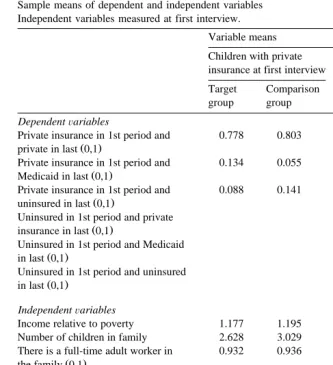
Table 2 provides the mean values for the dependent and independent variables used in the six models. Each dependent variable is an indicator for a child’s health insurance status at the last interview of the 1990 SIPP panel given their health insurance status at the first interview of the panel. We focus only on those children

Ž

who were not enrolled in the Medicaid program i.e., were privately insured or

.

uninsured prior to the time the children’s expansions were mandated, as these are the children who may have been influenced to enroll in Medicaid due to the expansions.

Seventy-eight percent of the target group children and 80% of the comparison group children who began the panel with private insurance also had private coverage at the last interview. Thirteen percent of the target group children starting in private had Medicaid coverage at the last interview while 9% was uninsured. This dynamics was reversed for the comparison group children, with 6% of those starting with private coverage having Medicaid in the last period and 14% being uninsured. Of those beginning the panel uninsured, 42% of the target children was also uninsured at the end as was 58% of the comparison group children. The remaining target group children were fairly evenly divided between those with

15

(15)

Table 2

Sample means of dependent and independent variables Independent variables measured at first interview.

Variable means

Children with private Children uninsured insurance at first interview at first interview Target Comparison Target Comparison

group group group group

DependentÕariables

Private insurance in 1st period and 0.778 0.803

Ž .

private in last 0,1

Ž .

Medicaid in last 0,1

Ž .

uninsured in last 0,1

Uninsured in 1st period and private 0.284 0.252

Ž .

insurance in last 0,1

Uninsured in 1st period and Medicaid 0.292 0.169

Ž .

in last 0,1

Uninsured in 1st period and uninsured 0.424 0.576

Ž .

in last 0,1

IndependentÕariables

Income relative to poverty 1.177 1.195 0.796 0.849

Number of children in family 2.628 3.029 2.503 2.875

There is a full-time adult worker in 0.932 0.936 0.776 0.865

Ž .

the family 0,1

Age of high-earning adult 30.873 35.077 30.187 34.875

High-earner has high school diploma 0.440 0.444 0.391 0.428

Ž .

only 0,1

High-earner has some college 0.400 0.373 0.268 0.232

Ž .

education 0,1

Ž .

Child is in a two-parent family 0,1 0.796 0.735 0.722 0.723

Ž .

High-earner’s race is white 0,1 0.798 0.774 0.797 0.756

Ž .

Child lives in the midwest 0,1 0.280 0.250 0.218 0.182

Ž .

Child lives in the south 0,1 0.365 0.387 0.460 0.526

Ž .

Child lives in the west 0,1 0.178 0.195 0.240 0.188

Sample size 968 717 509 393

private insurance and those with Medicaid at the last interview. Of the comparison group children, 25% who started the panel uninsured had private coverage at the end and 17% had Medicaid coverage.

(16)

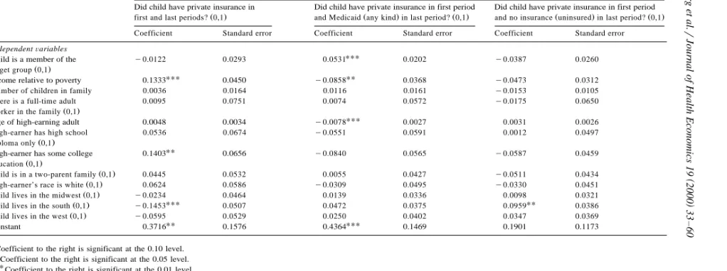
5.1. Insurance status at last interÕiew conditional on haÕing priÕate insurance coÕerage at first interÕiew

Table 3 provides the results for the set of models that includes only those children who had private insurance at the first interview. Being in the target group

Žchildren within the age and income constraints for Medicaid expansion eligibility.

is negatively associated with having private insurance in both the first and last

Ž .

interviews of the panel bs y0.0122 . This implies that there is a difference in probability ofy1.2 percentage points between the target and comparison groups. The negative coefficient on the target variable implies that some children may have left private coverage as a simple result of the expansions. The estimated difference was not, however, statistically significant, which may be an artifact of the low statistical power noted earlier.16

Being in the target group increases the probability that a child will make a private-to-Medicaid transition by 5.3 percentage points, an effect that is statisti-cally significant at the 0.01 level. Being in the target group lowers the probability of a transition from private insurance to uninsurance at the end of the panel by 3.9 percentage points, a difference that is not statistically significant.17

To summarize the results of the first set of multivariate models, being a child in the age and income groups targeted by the Medicaid expansions:

Ø lowers the probability that a child with private coverage at the first interview also has private coverage at the last interview;

Ø increases the probability that a child with private coverage at the first interview has Medicaid coverage at the last interview; and

Ø decreases the probability that a child with private coverage at the first interview is uninsured at the last interview.

The negative coefficient on ‘target’ in the equation predicting whether a child would have private coverage in the first and last interviews of the survey indicates that some displacement of private coverage may have occurred for those children who had private coverage at the beginning of the panel. How important is this displacement? Clearly, not all transitions from private coverage to Medicaid coverage during this period were attributable to ‘‘crowd-out’’. Some children who

16

Given our sample size, in order to have an 80% probability of detecting a significant difference between the target and comparison groups in the probability of being in private in the last period, the actual difference between the two populations would have to be at least 5.1 percentage points in comparison to the current 1.2 percentage points. In order to have an 80% probability of detecting a difference of 1.2 percentage points as being statistically significant, the sample size for the target and comparison groups would have to be approximately 17,000.

17

The 3 percentage point differences across the three models do not sum exactly to zero because

Ž

there were a small number of private coverage to non-Medicaid public coverage transitions e.g.,

.

(17)

()

Sample used in estimation includes those children in the target and comparison groups who had private insurance at the first interview. Standard errors adjusted for clustering within family units and SIPP complex sampling design.

Independent variables are measured at first interview.

Ž .

Income relative to poverty reflects definition of income used to determine Medicaid eligibility i.e., income less disregards . Dependent variables

Did child have private insurance in Did child have private insurance in first period Did child have private insurance in first period

Ž . Ž . Ž . Ž . Ž .

first and last periods? 0,1 and Medicaid any kind in last period? 0,1 and no insurance uninsured in last period? 0,1 Coefficient Standard error Coefficient Standard error Coefficient Standard error

UUU

Child is a member of the y0.0122 0.0293 0.0531 0.0202 y0.0387 0.0260

Ž . target group 0,1

UUU UU

Income relative to poverty 0.1333 0.0450 y0.0858 0.0368 y0.0473 0.0312

Number of children in family 0.0036 0.0164 0.0116 0.0161 y0.0153 0.0105

There is a full-time adult 0.0095 0.0751 0.0074 0.0572 y0.0175 0.0650

Ž . worker in the family 0,1

UUU

Age of high-earning adult 0.0048 0.0034 y0.0078 0.0027 0.0031 0.0026

High-earner has high school 0.0536 0.0674 y0.0551 0.0591 0.0012 0.0497

Ž . diploma only 0,1

UU

High-earner has some college 0.1403 0.0656 y0.0840 0.0565 y0.0587 0.0459

Ž . education 0,1

Ž .

Child is in a two-parent family 0,1 0.0445 0.0532 0.0055 0.0427 y0.0511 0.0434

Ž .

High-earner’s race is white 0,1 0.0624 0.0586 y0.0309 0.0495 y0.0330 0.0451

Ž .

Child lives in the midwest 0,1 y0.0234 0.0464 0.0139 0.0336 0.0098 0.0321

UUU UU

Ž .

Child lives in the south 0,1 y0.1453 0.0507 0.0472 0.0375 0.0959 0.0386

Ž .

Child lives in the west 0,1 y0.0595 0.0529 0.0250 0.0402 0.0347 0.0369

UU UUU

Constant 0.3716 0.1576 0.4364 0.1469 0.1901 0.1173

U

Coefficient to the right is significant at the 0.10 level.

UU

UUU

(18)

moved into Medicaid from private coverage would have been uninsured in the absence of the expansions, as the recession and other unrelated trends in health insurance coverage which occurred over the same period decreased the overall level of private health insurance coverage.

To answer this question, we divide the decreased probability attributable to the expansions that a child would have private coverage in both the first and last

Ž .

periods by the increased probability also attributable to the expansions that a child would have private coverage in the first period but Medicaid coverage in the last period. The resulting calculation, which uses the probabilities shown in Table

Ž .

3 y0.0122r0.0531s y0.2298 , implies that 23% of these private-insurance-to-Medicaid transitions attributable to the expansions was made by children who

Ž .

otherwise would have had private insurance coverage standard errors0.55 . This estimate focuses exclusively on change over a 28-month period, ignoring short-term transitions that may have occurred in the interim or following the end of the panel. Thus, even if the estimated coefficients on the ‘target’ variable reflect a real crowd-out effect that the small sample size is preventing from being statistically

Ž

significant, the magnitude of the point estimate is relatively small i.e., 77% of the private coverage to Medicaid transitions was not attributable to those who would

.

have been privately insured in the absence of the expansions .

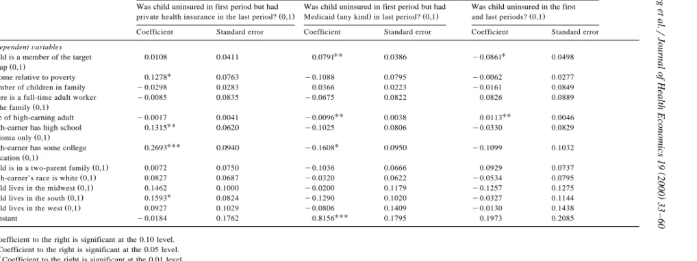
5.2. Insurance status at last interÕiew conditional on being uninsured at first interÕiew

Table 4 provides the results for children who were uninsured at the first interview. Being in the target group implies a higher probability of moving from

Ž .

uninsurance to private coverage bs0.0108 , a relationship that is not statisti-cally significant but certainly gives no sign of any crowd-out. The fact that target children were not less likely to move out of uninsurance and into private coverage

Žand might be more likely to do so indicates that uninsured children were not.

opting for Medicaid coverage as opposed to moving into private insurance. The probability of moving from being uninsured to Medicaid coverage was also higher for those in the target group, as one would expect, with a difference of 7.9 percentage points between the target and comparison groups which is statistically significant at the 0.05 level. Being in the target group lowers the probability that a

Ž .

child uninsured at the first interview was uninsured at the last bs y0.0861 , a modestly significant result.

To summarize the results of the second set of multivariate models, being a child in the age and income groups targeted by the Medicaid expansions:

Ø increases the probability that a child who was uninsured at the first interview had private coverage at the last interview;

Ø increases the probability that a child who was uninsured at the first interview had Medicaid at the last interview; and

(19)

()

Samples used in estimation includes those children in the target and comparison groups who were uninsured at the first interview. Standard errors adjusted for clustering within family units and SIPP complex sampling design.

Ž .

Was child uninsured in first period but had Was child uninsured in first period but had Was child uninsured in the first

Ž . Ž . Ž . Ž .

private health insurance in the last period? 0,1 Medicaid any kind in last period? 0,1 and last periods? 0,1

Coefficient Standard error Coefficient Standard error Coefficient Standard error

UU U

Child is a member of the target 0.0108 0.0411 0.0791 0.0386 y0.0861 0.0498

Ž . group 0,1

U

Number of children in family y0.0298 0.0283 0.0366 0.0223 y0.0161 0.0849

There is a full-time adult worker y0.0085 0.0835 y0.0675 0.0822 0.0826 0.0889

Ž . in the family 0,1

UU UU

Age of high-earning adult y0.0017 0.0041 y0.0096 0.0038 0.0113 0.0046

UU

High-earner has high school 0.1315 0.0620 y0.1025 0.0806 y0.0330 0.0829

High-earner has some college 0.2693UUU _0.0940 _y_0.1608U _0.0950 _y_0.1099 _0.1032

Ž . education 0,1

Ž .

Child is in a two-parent family 0,1 0.0072 0.0750 y0.1036 0.0666 0.0929 0.0737

Ž .

Child lives in the midwest 0,1 0.1462 0.1000 y0.0200 0.1179 y0.1257 0.1275

U

Ž .

Child lives in the south 0,1 0.1593 0.0824 y0.1290 0.1020 y0.0327 0.1144

Ž .

Child lives in the west 0,1 0.0927 0.1029 y0.0806 0.1409 y0.0130 0.1438

UUU

Constant y0.0184 0.1762 0.8156 0.1795 0.1973 0.2085

U

UU

UUU

(20)

These estimates provide no support for the conclusion that the Medicaid expansions displaced private coverage for those children who were uninsured prior to the implementation of the program mandates. In fact, there is some weak evidence that those initially uninsured in the target group transitioned to private coverage in greater proportions than their comparison group counterparts.

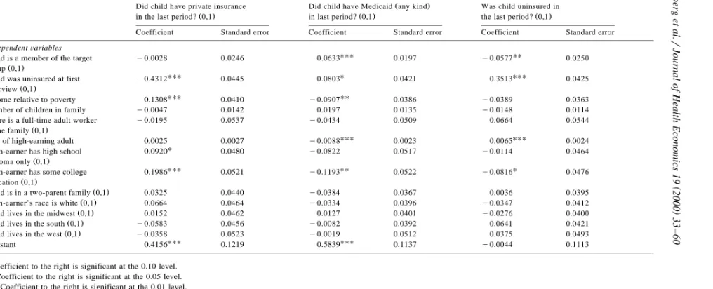
5.3. Combined effect for children in priÕate coÕerage or uninsured at first interÕiew

We next estimated a set of models which would generate a combined estimate of the effects of the expansions on private coverage for children who had either private coverage or were uninsured the first interview of the SIPP panel. The results of these models are presented in Table 5. Being in the target group has a negative but statistically insignificant effect on the probability that a child had private insurance in the last period. The difference in probability between the target and comparison groups was approximately 0.3 percentage points. Being in the target group had a positive and highly significant effect on the probability that a child would have Medicaid coverage in the last period of the panel, with the difference in probability equal to 6.3 percentage points. In addition, being in the target group had a negative and significant effect on the probability that a child would be uninsured at the end of the SIPP panel, with target children being 5.6 percentage points less likely to be uninsured than the comparison children.

Taking the ratio of the coefficients for the target variables in the first two equations, as we have done in the previous set of models, yields an overall estimate of the Medicaid expansion displacement effect. In this way, we estimate

Ž .

that 4.4% y0.0028r0.0633 of the children who moved into Medicaid from either private coverage or uninsurance over the course of the SIPP panel would

Ž

have had private coverage in the absence of the expansions standard error is

. 18

0.38 . This result, in effect, averages the two independent results calculated

18

In order to increase our sample size, we considered including children up to age 13 in our analysis. However, there are differences in health care utilization patterns and the consequent demand for health insurance between younger and older children. Therefore, we would expect that the older the children included in the comparison group, the less comparable the two groups would be. In addition, we want to avoid including pregnant teenagers in our comparison group because they were affected by the Medicaid expansions for pregnant women. The older the child, the higher the probability of pregnancy. We did, however, test the sensitivity of our results to the inclusion of children who were 13 and younger at the start of the panel. This change leads to an overall crowd-out estimate of 14.9% as compared to 4.4%. The crowd-out effect for the group beginning the panel in private coverage was

Ž .

y40.7% y0.024r0.0589, as compared to 23% ; the effect for the group beginning the panel

Ž .

(21)

()

Sample used in estimation includes those children in the target and comparison groups who had private insurance or were uninsured at the first interview. Standard errors adjusted for clustering within family units and SIPP complex sampling design.

Ž .

Did child have private insurance Did child have Medicaid any kind Was child uninsured in

Ž . Ž . Ž .

in the last period? 0,1 in last period? 0,1 the last period? 0,1

UUU UU

Child is a member of the target y0.0028 0.0246 0.0633 0.0197 y0.0577 0.0250

Ž . group 0,1

UUU U UUU

Child was uninsured at first y0.4312 0.0445 0.0803 0.0421 0.3513 0.0425

Ž . interview 0,1

UUU UU

UUU UUU

U

UUU UU U

Ž . education 0,1

Ž .

Child is in a two-parent family 0,1 0.0325 0.0440 y0.0384 0.0367 0.0036 0.0395

Ž .

Child lives in the midwest 0,1 0.0152 0.0462 0.0127 0.0401 y0.0276 0.0400

Ž .

Child lives in the south 0,1 y0.0583 0.0456 y0.0082 0.0392 0.0641 0.0421

Ž .

Child lives in the west 0,1 y0.0358 0.0523 y0.0019 0.0512 0.0375 0.0493

UUU UUU

Constant 0.4156 0.1219 0.5839 0.1137 y0.0044 0.1113

U

UU

UUU

(22)

earlier from the two separate samples conditional on initial insurance coverage. Consistent with those results, this overall estimate takes into account both the negative and insignificant effect seen from the sample of children beginning the panel in private coverage and the positive and insignificant effect seen from the sample of children beginning the panel uninsured.

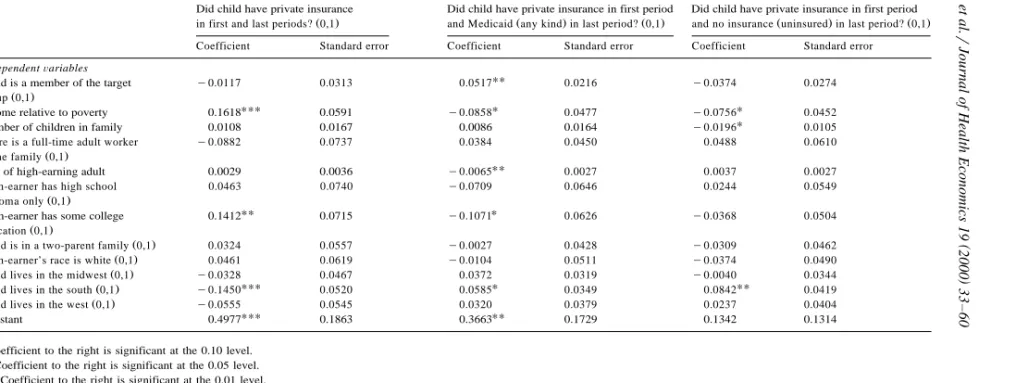
5.4. Children with Medicaid eligibility under non-expansion rules at first interÕiew

Some children in our sample would have been eligible for Medicaid at the first interview even in the absence of the expansions through the Ribicoff, DEFRA or medically needy provisions.19 _{To the extent that these children behave differently}

Ž .

from the higher-income children eligible for Medicaid due only to the expan-sions — and to the extent that they are differentially represented among the target and comparison groups — their inclusion could affect the direct applicability of our results to the Medicaid expansions themselves. For example, the fact that these children were eligible under previous Medicaid rules but did not participate in the program may simply indicate that their families do not have strong preferences regarding insurance coverage. We tested the sensitivity of our results to the inclusion of these children by performing a re-estimation without them.

This re-estimation had virtually no effect on the probability of any particular

Ž

last period status for those with private insurance at the first interview see Table

.

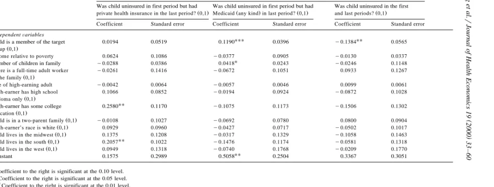
6 , nor did it affect the probability that a child would move from being uninsured to having private insurance over the 28-month period. However, the re-estimation did make a difference in the estimated probabilities of having Medicaid or being uninsured in the last period for those who were uninsured at the first interview

Žsee Table 7 ..

The probability that a child in the target group would move from being uninsured at the first interview to having Medicaid at the last period increased

Ž .

from a bs0.0791 significant at the 0.05 level for the broader sample of

Ž .

children to bs0.1190 significant at the 0.01 level for the smaller sample of children. This implies that children who were uninsured and non-Medicaid-eligible at the first interview and became eligible through the Medicaid expansions were 12 percentage points more likely to have Medicaid at the last interview than similar children in the comparison group.

Similarly, the smaller sample estimates imply that children in the expansion-eligible group were 14 percentage points less likely than the comparison group children to be uninsured at both the first and the last interviews, a result which was

19

For a full discussion of the legislative history and details regarding these other eligibility routes,

Ž .

(23)

()

Sample used in estimation includes those children in the target and comparison groups who had private coverage at the first interview. Standard errors adjusted for clustering within family units and SIPP complex sampling design.

Ž .

Did child have private insurance Did child have private insurance in first period Did child have private insurance in first period

Ž . Ž . Ž . Ž . Ž .

in first and last periods? 0,1 and Medicaid any kind in last period? 0,1 and no insurance uninsured in last period? 0,1 Coefficient Standard error Coefficient Standard error Coefficient Standard error

UU

Child is a member of the target y0.0117 0.0313 0.0517 0.0216 y0.0374 0.0274

Ž . group 0,1

UUU U U

U

Number of children in family 0.0108 0.0167 0.0086 0.0164 y0.0196 0.0105

There is a full-time adult worker y0.0882 0.0737 0.0384 0.0450 0.0488 0.0610

UU

High-earner has high school 0.0463 0.0740 y0.0709 0.0646 0.0244 0.0549

UU U

Ž . education 0,1

Ž .

Child is in a two-parent family 0,1 0.0324 0.0557 y0.0027 0.0428 y0.0309 0.0462

Ž .

Child lives in the midwest 0,1 y0.0328 0.0467 0.0372 0.0319 y0.0040 0.0344

UUU U UU

Ž .

Child lives in the south 0,1 y0.1450 0.0520 0.0585 0.0349 0.0842 0.0419

Ž .

Child lives in the west 0,1 y0.0555 0.0545 0.0320 0.0379 0.0237 0.0404

UUU UU

Constant 0.4977 0.1863 0.3663 0.1729 0.1342 0.1314

U

UU

UUU

(24)

()

Results of linear probability models including children who were uninsured at first interview: sample excludes children eligible for Medicaid through non-expansion routes of eligibility at first interview

Number of observations is 650.

Sample used in estimation includes those children in the target and comparison groups who were uninsured at the first interview. Standard errors adjusted for clustering within family units and SIPP complex sampling design.

Ž .

Was child uninsured in first period but had Was child uninsured in first period but had Was child uninsured in the first

Ž . Ž . Ž . Ž .

private health insurance in the last period? 0,1 Medicaid any kind in last period? 0,1 and last periods? 0,1

UUU UU

Child is a member of the target 0.0194 0.0519 0.1190 0.0396 y0.1384 0.0565

Ž . group 0,1

U

Age of high-earning adult y0.0042 0.0064 y0.0057 0.0046 0.0099 0.0061

High-earner has some college 0.2580UU _0.1170 _y_0.1075 _0.1173 _y_0.1506 _0.1302

Ž . education 0,1

Ž .

Child is in a two-parent family 0,1 y0.0108 0.1027 y0.0692 0.0780 0.0800 0.0904

Ž .

Child lives in the midwest 0,1 0.1375 0.1208 y0.0317 0.1329 y0.1058 0.1463

UU

Ž .

Child lives in the south 0,1 0.2057 0.1022 y0.1476 0.1174 y0.0581 0.1318

Ž .

Child lives in the west 0,1 0.0949 0.1318 y0.0740 0.1768 y0.0209 0.1770

UU

Constant 0.1575 0.2989 0.5058 0.2504 0.3367 0.3051

U

UU

UUU

(25)

Ž .

significant at the 0.05 level . The magnitude of this effect was roughly 60% higher than that of the effect estimated with the larger sample.

To summarize, limiting the sample to those children who were either not eligible for Medicaid at the first interview or who were eligible only as a result of the expansions strengthens two of our major conclusions. First, it increases the probability of expansion-eligible children who were uninsured at the first inter-view moving to Medicaid. Second, it decreases the probability that expansion-eligible children who were uninsured at the beginning were still uninsured at the end of the 28-month period.

6. Conclusions

In this analysis, we use longitudinal data from the 1990 panel of the SIPP to estimate the extent of crowd-out resulting from the Medicaid expansions for children implemented during the early 1990s. We find that 23% of the expansion-related movement from private coverage to the Medicaid program was attributable to families choosing Medicaid coverage who would have been covered by private insurance in the absence of the expansions. We find no evidence that the Medicaid expansions encouraged families with uninsured children to enroll their children in Medicaid rather than take up private coverage. These results imply that the primary impact of the Medicaid expansions was to prevent low-income children from becoming or remaining uninsured, not to crowd-out private insurance.

This paper raises important questions about the feasibility of using currently available longitudinal data to assess the extent to which expansions of public programs that affect only a small portion of the population displace private insurance coverage. While the SIPP is the largest nationally representative longitu-dinal dataset that can be used to study this issue either under the Medicaid

Ž .

(26)

we present here.20 Consequently, while we do not consider these results to be definitive, we feel they are a relevant contribution to the ongoing debate regarding the interplay between public and private insurance coverages.

6.1. ReleÕance for CHIP

With regard to current policy issues and debates, it is difficult to extrapolate the results of this analysis to the new CHIP due to three programmatic differences. First, the fiscal implications of crowd-out under the CHIP program are likely to be greater than under the Medicaid expansions. This is because children eligible for CHIP will, by definition, have higher family incomes than children eligible for the Medicaid expansions in their state. As income increases, the probability that a child has private insurance increases and thus, the probability that a child is uninsured decreases. Therefore, even if children eligible under CHIP leave private coverage at the same rate as children under the expansions did, and even if uninsured children participate at the same rate as uninsured children eligible under the expansions, the proportion of new entrants into the program who previously had private coverage is likely to be higher than under the expansions.

The second potential difference is the structure of CHIP programs. States have the option to implement their CHIP coverage expansions through Medicaid or through other state-designed plans. Depending upon the structural program choices that states make, the participation rates among both the previously privately insured and the uninsured could vary substantially from those under the expan-sions, with important implications for the magnitude of displacement. The third difference is that states are required to develop strategies for reducing crowd-out under the CHIP program. The effectiveness of these preventive approaches is, of course, still unknown.

The crowd-out issue has the opportunity to focus the debate over how society will evaluate the success of public insurance programs. On one hand is the goal of

Ž .

minimizing the public cost per newly insured individual target efficiency . On the other hand is the goal of providing public income support in such a way that people in similar economic circumstances receive similar levels of assistance

Ž_{horizontal equity . The concern with crowd-out, per se, touches only upon the}.

20

In fact, our results are consistent with those produced by Thorpe and Florence using the NLSY, although not directly comparable since Thorpe and Florence examine all movements into Medicaid while we examine expansion-related movement into Medicaid. A rough check on the consistency of the two studies can be made by focusing on movements from private coverage to Medicaid coverage for

Ž

children with incomes above 100% of poverty who would have only been eligible due to the

.

(27)

efficiency with which a program targets public dollars to the previously uninsured. While target efficiency is a relevant and important component of judging the cost-effectiveness of particular programs, it is not the only criterion against which new programs need to be evaluated.

The attention that the crowd-out debate has engendered at both the state and federal levels highlights the need for explicit prioritization of public insurance program goals and the design of program evaluations consistent with those priorities. Unless the often-competing goals of target efficiency of public dollars, equity of income redistribution, high participation rates, access to high quality medical care, and continuity of insurance coverage are considered relative to one another, not in isolation, we cannot hope to design public programs to meet the health care needs society has identified.

Acknowledgements

This work was funded by a grant from the Robert Wood Johnson Foundation. The authors are grateful for the helpful advice of John Holahan, Robert Kaestner, Genevieve Kenney, John Marcotte, Len Nichols, Doug Wissoker, and Steve Zuckerman. In addition, we appreciate the suggestions and guidance of David Cutler, Jonathon Gruber, Joseph Newhouse, and two anonymous referees during the review process.

References

Ž

Congressional Research Service, 1993, Medicaid source book: background data and analysis a 1993

.

update . A report prepared by the Congressional Research Service for the use of the Subcommittee on Health and the Environment of the Committee on Energy and Commerce, U.S. House of Representatives.

Cutler, D.M., Gruber, J., 1996a. Does public insurance crowd-out private insurance?. Quarterly Journal

Ž .

of Economics 111 2 , 391–430.

Cutler, D.M., Gruber, J., 1996b. The effect of Medicaid expansions on public insurance, private

Ž .

insurance and redistribution. American Economic Review 86 2 , 378–383.

Dubay, L.C., 1999. Expansions in public health insurance and crowd-out: what the evidence says. In: Options for Expanding Health Insurance Coverage: What Difference Do Different Approaches Make? Background Papers, Henry J. Kaiser Family Foundation Project on Incremental Health Reform.

Dubay, L.C., Kenney, G.M., 1996. Revisiting the issues: the effects of Medicaid expansions on

Ž .

insurance coverage of children. The Future of Children 6 1 , 152–161.

Dubay, L.C., Kenney, G.M., 1997. Did Medicaid expansions for pregnant women crowd-out private

Ž .

insurance?. Health Affairs 16 1 , 185–193.

Dubay, L.C., Kenney, G.M., Norton, S.A., Cohen, B.C., 1995. Local responses to expanded Medicaid

Ž .

coverage for pregnant women. Milbank Quarterly 73 4 , 535–563.

(28)

Hill, I., 1992. The Medicaid expansions for pregnant women and children: a state program character-istics information base. Health Systems Research, Washington, DC.

Holahan, J., Winterbottom, C., Rajan, S., 1995. The changing composition of health insurance

Ž .

coverage in the United States. Health Affairs 14 4 , 253–264.

Huber, P.J., 1967. The behavior of maximum likelihood estimates under non-standard conditions. In: Proceedings of the Fifth Berkeley Symposium in Mathematical Statistics and Probability. Univer-sity of California Press, Berkeley, CA, pp. 221–233.

Kasper, J.D., 1987. The importance of type of usual source of care for children’s physician access and

Ž .

expenditures. Medical Care 25 5 , 386–398.

Leftkowitz, D.C., Short, P.F., 1989. Medicaid eligibility and the use of preventive services by low-income children. Paper presented at the 1989 Annual Meeting of the American Public Health Association, Chicago, IL.

Rosenbach, M.L., 1985. Insurance coverage and ambulatory medical care of low-income children: United States, 1980. Reports from the National Medical Care Utilization and Expenditure Survey, Series C, Analytical Report No. 1. U.S. Department of Health and Human Services, Public Health Service, National Center for Health Statistics, Washington, DC.

Shore-Sheppard, L., 1997. Stemming the tide: the effect of expanding Medicaid eligibility on health insurance coverage. University of Pittsburgh Working Paper, November.

Short, P.F., Leftkowitz, D.C., 1991. Encouraging preventive services for low-income children: the effect of expanding Medicaid. Paper presented at the 1991 Annual Meeting of the Association for Health Services Research, San Diego, CA.

Thorpe, K.E., Florence, C., 1998. Health insurance coverage among children: the role of expanded

Ž .

Medicaid coverage. Inquiry 35 4 , 369–379.

White, H., 1980. A heteroskedasticity-consistent covariance matrix estimator and a direct test for heteroskedasticity. Econometrica 48, 817–830.

Yazici, E.Y., Kaestner, R., forthcoming. Medicaid expansions and the crowding-out of private health insurance. Inquiry.