El e c t ro n ic
Jo ur n
a l o
f P
r o b
a b i l i t y
Vol. 13 (2008), Paper no. 23, pages 671–755. Journal URL
http://www.math.washington.edu/~ejpecp/
Convergence of lattice trees to super-Brownian
motion
above the critical dimension
Mark Holmes∗ Department of Statistics The University of Auckland
Private Bag 92019 Auckland 1142
New Zealand
Email: [email protected]
Abstract
We use the lace expansion to prove asymptotic formulae for the Fourier transforms of the r-point functionsfor a spread-out model of critically weighted lattice trees inZd
ford >8. A lattice tree containing the origin defines a sequence of measures onZd
, and the statistical mechanics literature gives rise to a natural probability measure on the collection of such lattice trees. Under this probability measure, our results, together with the appropriate lim-iting behaviour for the survival probability, imply convergence to super-Brownian excursion in the sense of finite-dimensional distributions .
Key words: Lattice trees, super-Brownian motion, lace expansion.
AMS 2000 Subject Classification: Primary 82B41, 60F05, 60G57, 60K35. Submitted to EJP on June 6, 2007, final version accepted April 3, 2008.
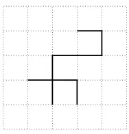
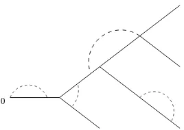
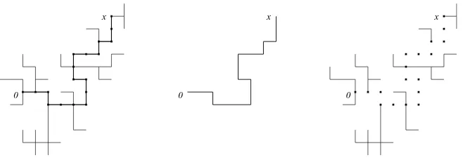
Figure 1: A nearest neighbour lattice tree in 2 dimensions.
1
Introduction
Alattice treeinZdis a finite connected set of bonds containing no cycles (see Figure 1). Lattice
trees are an important model for branched polymers. They are of interest in statistical physics, and perhaps combinatorics and graph theory. We expect that our results are also appealing to probabilists, since there is a critical lattice tree weighting scheme and a corresponding sequence of measures that are believed to converge (in dimensions d > 8) to the canonical measure of super-Brownian motion, a well-known measure in the superprocesses literature. The main result of this paper establishes asymptotic formulae for the Fourier transforms of the so-calledr-point functions, which goes part way to proving this convergence result. The 2-point functiontn(x),
is (up to scaling) the probability that a (critically weighted) random lattice tree containing the origin, also contains the pointx∈Zd at tree-distancenfrom the origin.
Lattice trees are self-avoiding objects by definition (since they contain no cycles). It is plausible that the self-avoidance constraint imposed by the model becomes less important as the dimension increases. Lubensky and Isaacson [23] proposeddc= 8 as the critical dimension for lattice trees
and animals, at which various critical exponents cease to depend on the dimension and take on their mean-field values (with log corrections when d = 8). Macroscopic properties of the model should be similar to a simpler model, called branching random walk, that does not have the self-avoidance constraint. A good source of information on critical exponents for lattice trees (self-avoiding branched polymers) is [7]. There are few rigorous results for lattice trees for 1 < d ≤ 8. The scaling limit of the model in 2 dimensions is not expected to be conformally invariant, so that the class of processes called Stochastic Loewner Evolution (SLE) (see for example [27]) is not a suitable candidate for the scaling limit. Brydges and Imbrie [3] used a dimensional reduction approach to obtain strong results for a continuum (i.e. not lattice based) model for d = 2,3. Appealing to universality, we would expect lattice trees to have the same critical exponents as the Brydges and Imbrie model.
In high dimensions much more is known. Letρpc(x) =
P
ntn(x). Hara and Slade [9], [10] proved
the finiteness of thesquare diagramPx,y,zρpc(x)ρpc(y−x)ρpc(z−y)ρpc(z) for sufficiently
spread-out lattice trees ford >8, and for the nearest neighbour model ford≫8. With van der Hofstad [8], they showed mean-field behaviour ofρpc(x) for a sufficiently spread-out model whend >8.
measure on Rd called integrated super-Brownian excursion (ISE). The ISE is essentially what
one gets from integrating super-Brownian excursion (whose law is the canonical measure of super-Brownian motion) over time and conditioning the resulting random measure to have total mass 1. In this paper the total mass is unrestricted and the temporal component of the trees and limiting process is retained.
Results of Hara and Slade (see for example [24]) show that ford >4, self-avoiding walk (SAW) converges to Brownian motion in the scaling limit. This is achieved by proving convergence of the finite-dimensional distributions and tightness. In this case tightness follows from a nega-tive correlation property of the model. Note that, almost surely, Brownian motion paths have Hausdorff dimension 2∧dand are self-avoiding in 4 or more dimensions.
With appropriate scaling of space, time, and mass, critical branching random walk converges weakly to super-Brownian motion (see for example [25]). One version of this statement is that µn =w⇒ N0 (as (sigma-finite) measures on the space D(MF(Rd)) of cadlag
finite-measure-valued paths on Rd), where µ
n ∈ MF(D(MF(Rd)) is an appropriate scaling of the law of the
correspondingly scaled branching random walk, andN0is a sigma-finite measure onD(MF(Rd)),
called the canonical measure of super-Brownian motion (CSBM). Denote byXta measure-valued
path with lawN0. The supports of the measuresY[t0,t1]=
Rt1
t0 Xsds and Y[t2,t3]=
Rt3
t2 Xsds have
no intersection in dimensionsd≥8 ift2 > t1 (N0-almost everywhere) [5]. This is the appropriate
way to say that SBM is self-avoiding for d ≥ 8. We might expect that critical lattice trees (described as a measure-valued process with appropriate scaling) converge weakly to CSBM in the same sense as branching random walk, for d >8.
In this paper we use the lace expansion to prove asymptotic formulae for the Fourier trans-forms of quantities called ther-point functions, for critical sufficiently spread-out lattice trees in dimensions d >8. Holmes and Perkins [21] prove that these formulae, together with an appro-priate asymptotic formula for the survival probability, imply convergence of the model to CSBM in the sense of finite-dimensional distributions. Tightness and the asymptotics of the survival probability remain open problems. Similar results have been obtained for critical spread-out models of oriented percolation [18], [13], [14] and the contact process [16] above their critical dimension (see also [11] and [12] for ordinary percolation). For a comprehensive introduction to the lace expansion and its applications up to 2005, see [26].
1.1 The model
We proceed to define the quantities of interest. We restrict ourselves to the vertex set of Zd.
Definition 1.1.
1. A bondis an unordered pair of distinct vertices in the lattice.
2. A cycle is a set of distinct bonds {v1v2, v2v3, . . . , vl−1vl, vlv1}, for some l≥3.
3. A lattice tree is a finite set of vertices and lattice bonds connecting those vertices, that contains no cycles. This includes the single vertex lattice tree that contains no bonds.
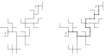
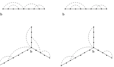
x
y
x
y
Figure 2: A nearest neighbour lattice tree in 2 dimensions. The backbone fromx toy of length
n= 17 is highlighted in the second figure.
connecting the xi. If r = 2 we often refer to the skeleton connecting x1 to x2 as the
backbone.
Remark 1.2. The nearest-neighbour model consists of nearest neighbour bonds {x1, x2} with
x1, x2 ∈Zd and|x1−x2|= 1. Figures 1 and 2 show examples of nearest-neighbour lattice trees
in Z2.
We useZ+ to denote the nonnegative integers{0,1,2, . . .}.
Definition 1.3.
1. For~x∈Zdl letT(~x) ={T :xi ∈T, i∈1, . . . , l}. Note that T(x) always includes thesingle
vertex lattice tree,T ={x} that contains no bonds.
2. For T ∈ T(o) we let Ti be the set of vertices x ∈ T such that the backbone from o to x consists ofi bonds. In particular for T ∈ T(o) we have To ={o}. A tree T ∈ T(o) is said tosurvive until time n if Tn6=∅.
3. For ˜x= (x1, . . . , xr−1) ∈Zd(r−1) and n˜ ∈Z+r−1 we we write ˜x∈Tn˜ if xi ∈Tni for each i and defineT˜n(x˜)≡ {T ∈ T(o) :˜x∈Tn˜}.
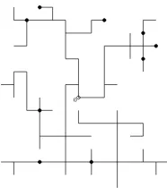
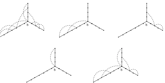
If we think of T ∈ T(o) as the path taken by a migrating population in discrete time, then Ti
can be thought of as the set of locations of particles alive at time i. Figure 3 identifies the set
T10 for a fixed T. Similarly Tn˜(˜x) can be thought of as the set of trees for which there is a
particle atxi alive at timeni for each i.
In order to provide a small parameter needed for convergence of the lace expansion, we consider trees consisting of bonds connecting vertices separated by distance at most L for some L≫1. Each bond is weighted according to a functionD, supported on [−L, L]dwith total mass 1. The methods and results in this paper rely heavily on the main results of [8] and [17]. Since the assumptions on the model are stronger in [8], we adopt the finite range L, D spread-out model of that paper. The following definition and the subsequent remark are taken, almost verbatim from [8].
Definition 1.4. Let h be a non-negative bounded function onRd which is piecewise continuous, symmetric under the Zd-symmetries of reflection in coordinate hyperplanes and rotation by π
0
Figure 3: A nearest neighbour lattice treeT in 2 dimensions with the setTi fori= 10.
supported in [−1,1]d, and normalised (R[−1,1]dh(x)ddx= 1). Then for large L we define
D(x) = P h(x/L)
x∈Zdh(x/L)
. (1.1)
Remark 1.5. Since Px∈Zdh(x/L) ∼ Ld using a Riemann sum approximation to
R
[−1,1]dh(x)ddx, the assumption thatLis large ensures that the denominator of (1.1) is non-zero.
Sinceh is bounded,Px∈Zdh(x/L)∼Ld also implies that
kDk∞≤ C Ld.
We defineσ2 =P
x|x|2D(x). The sum
P
x|x|rD(x) can be regarded as a Riemann sum and is asymptotic to a multiple ofLr for r >0. In particularσ andL are comparable. A basic example obeying the conditions of Definition 1.4 is given by the function h(x) = 2−dI[−1,1]d(x) for which
D(x) = (2L+ 1)−dI[−L,L]d∩Zd(x).
Definition 1.6 (L, D spread-out lattice trees). Let ΩD ={x ∈Zd :D(x) >0}. We define an
L, D spread-out lattice tree to be a lattice tree consisting of bonds{x, y} such thaty−x∈ΩD.
The results of this paper are for L, D spread-out lattice trees in dimensions d > 8. Appealing to the hypothesis of universality, we expect that the results also hold for nearest-neighbour lattice trees. However from this point on, unless otherwise stated, “lattice trees” and related terminology refers toL, D spread-out lattice trees.
Definition 1.7 (Weight of a tree). Given a finite set of bonds B and a nonnegative parameter
p, we define the weight of B to be
Wp,D(B) =
Y
{x,y}∈B
pD(y−x),
withWp,D(∅) = 1. If T is a lattice tree we define
Wp,D(T) =Wp,D(BT),
Definition 1.8 (ρ(x)). Let
ρp(x) =
X
T∈T(x)
Wp,D(T).
Clearly we haveρp(o) ≥1 for all L, psince the single vertex lattice tree{o}contains no bonds
and therefore has weight 1. A standard subadditivity argument [22] shows that there is a finite, positive pc at which Pxρp(x) converges for p < pc and diverges for p > pc. Hara, van der
Hofstad and Slade [8] proved the following Theorem, in whichO(y) denotes a quantity that is bounded in absolute value by a constant timesy.
Theorem 1.9. Let d >8 and fixν >0. There exists a constantA (depending on dandL) and anL0 (depending on d and ν) such that for L≥L0,
ρpc(x) =
A σ2(|x| ∨1)d−2
"
1 +O
Ã
L(d−8)∧2
(|x| ∨1)((d−8)∧2)−ν
!
+O
µ
L2
(|x| ∨1)2−ν
¶#
. (1.2)
Constants in the error terms are uniform in bothx andL, andA is bounded above uniformly in
L.
We henceforth take our trees at criticality and write
W(·) =Wpc,D(·), and ρ(x) =ρpc(x). (1.3)
It was also shown in [8] that pcρ(o)≤1 +O¡L−2+ν¢ and
ρ(x)≤C
Ã
Ix=0+
Ix6=0
L2−ν(|x| ∨1)d−2
!
, (1.4)
where the constants in the above statements depend onν andd, but notL.
1.2 The r-point functions
In this section we define the main quantities of interest in this paper, ther-point functions, and state the main results.
Definition 1.10 (2-point function). Forζ ≥0, n∈N, and x∈Rd we define,
tn(x;ζ) =ζn
X
T∈Tn(o,x)
W(T). (1.5)
We also define tn(x) =tn(x; 1).
Definition 1.11(Fourier Transform). Given an absolutely summable functionf :Zd(r−1)→R,
we let fb(k) =Px1,...,xr−1eiPjr−=11kj·xjf(~x) denote the Fourier transform of f (k
j ∈[−π, π]d).
In [17] the authors show that if a recursion relation of the form
fn+1(k;z) =
n+1
X
m=1
holds, and certain assumptions S, D, E, and G on the functions f•,g• and e• hold, then there exists a critical valuezcofzsuch thatfn(k, zc) (appropriately scaled) converges (up to a constant
factor) to the Fourier transform of the Gaussian density as n −→ ∞. In [15] this result is extended by generalizing assumptions E and G according to a parameter θ > 2, where the special case θ = d/2 with d > 4 is that which is proved in [17]. In Section 3.1 we show that
b
tn(k;ζ) obeys the recursion relation
btn+1(k;ζ) =
n+1
X
m=1
b
πm−1(k;ζ)ζpcDb(k)btn+1−m(k;ζ) +πbn+1(k;ζ),
whereπm(x;ζ) is a function that is defined in Section 3.1. After massaging this relation
some-what, the important ingredients in verifying assumptions E and G for our lattice trees model are bounds on bπm using information about ρ(x) andbtl(k;ζ) for l < m. The quantities πbm−1(k;ζ)
are reformulated using a technique known as thelace expansion, which is discussed in Section 2 and ultimately reduces the problem to one of studying certain Feynman diagrams. As in some of the references already discussed, the critical dimension dc = 8 appears in this analysis as the
dimension above which thesquare diagram
ρ(4)(o) = X
x,y,z
ρ(x)ρ(y−x)ρ(z−y)ρ(z)
converges.
The parameter ζ appears in (1.10) as an additional weight on bonds in the backbone of trees
T ∈ Tn(x). Those trees are already critically weighted bypc (a weight present on everybond in
the tree) as described by Definition 1.7 and (1.3) and exhibit mean-field behaviour in the form of Theorem 1.9. One might therefore expect a Gaussian limit forbtn with ζ = 1. The following
theorem is proved using the induction approach of [15], together with a short argument showing that the critical value ofζ obtained from the induction isζc = 1.
Theorem 1.12. Fix d >8, t >0, γ ∈ (0,1∧d−28) and δ ∈(0,(1∧d−28)−γ). There exists a positive L0 =L0(d) such that: For every L ≥L0 there exist positive A and v depending on d
and L such that
b
t⌊nt⌋
µ
k
√
vσ2n
=Ae−|k|
2 2d t+O
µ
|k|2
n
+O
µ
|k|2t1−δ
nδ
+O
Ã
1
(nt∨1)d−28
!
,
with the error estimate uniform in ©k∈Rd:|k|2 ≤Ct−1log(⌊nt⌋ ∨1)ª, where C = C(γ) and
the constants in the second and third error terms may depend on L.
More generally, we consider lattice trees containing the origin and r−1 other fixed points at fixed times.
Definition 1.13 (r-point function). For r≥3,n˜∈Nr−1 andx˜∈Rd(r−1) we define
tr˜n(˜x) =
X
T∈T˜n(˜x)
0 1 2 1 0
3 2
1
0 2
2 3
3
1 1
0 0
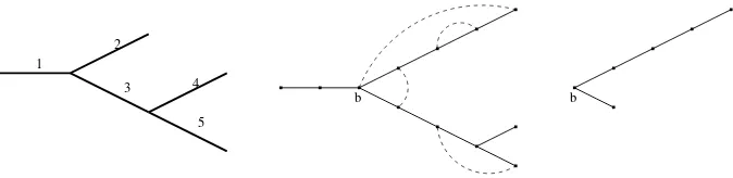
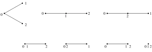
Figure 4: The unique shapeα(r) for r= 2,3 and the 3 shapes for r= 4.
To state a version of Theorem 1.12 forr-point functions forr >3 we need the notion ofshapes, which are abstract (partially labelled) sets of vertices and edges connecting those vertices, with special binary tree topologies.
The degree of a vertex v is the number of edges incident to v. Vertices of degree 1 are called leaves. Vertices of degree ≥ 3 are called branch points. There is a unique shape for r = 2 consisting of 2 vertices (labelled 0, 1) connected by a single edge. The vertex labelled 0 is called the root. For r ≥3 we have Qrj=3(2j−5)r-shapes obtained by adding a vertex to any of the 2(r−1)−3 edges of each (r−1)-shape, and a new edge to that vertex. The leaf of this new edge is labelled r−1. Each r-shape has 2r−3 edges, labelled in a fixed but arbitrary manner as 1, . . . ,2r−3. This is illustrated in figure 4 which shows the shapes for r = 2,3,4. Let Σr
denote the set ofr-shapes. By convention, the edges inα∈Σr are directed away from the root.
By construction eachr-shape hasr−2 branch points, each of degree 3.
Given a shape α ∈Σr and ˜k∈R(r−1)d we define ~κ(α)∈R(2r−3)d as follows. For each leaf j in
α (other than 0) we let Ej be the set of edges in α of the unique path in α from 0 to j. For
l= 1, . . . ,2r−3, we define
κl(α) = r−1
X
j=1
kjI{l∈Ej}. (1.8)
Next, givenα and~s∈R(2+r−3) we defineς˜(α)∈R(+r−1) by
ςj(α) =
X
l∈Ej
sl.
Finally we define
R˜t(α) ={~s:˜ς(α) =˜t}.
This is an (r−2)-dimensional subset ofR(2+r−3). For r= 3 we simply have
R˜t(α) ={(s, t1−s, t2−s) :s∈[0, t1∧t2]}.
It is known [1] that forr≥2, 0< t1< t2· · ·< tr−1 andφk(x) =eik·x,
EN0
rY−1
j=1
Xtj(φkj)
= X
α∈Σr
Z
R˜t(α) 2Yr−3
l=1
e−κl(α2d)2sld~s, (1.9)
where Xt(φ) ≡ R φ(x)Xt(dx), and EN0 denotes integration with respect to the sigma-finite measure N0. Forr= 3 this reduces to
Z t1∧t2
0
e−(k1+k2)
2s 2d e−
k1 (2t1−s) 2d e−
k22 (t2−s)
Theorem 1.14. Fix d >8, and δ∈(0,(1∧d−28)). There exists L0 =L0(d)≫1 such that: for
each L ≥ L0 there exists V = V(d, L) > 0 such that for every ˜t ∈ (0,∞)(r−1), r ≥ 3, K > 0,
and k˜kk∞≤ K,
b
tr
⌊n˜t
⌋
Ã
˜ k
√
vσ2n
!
=nr−2Vr−2A2r−3
" X
α∈Σr
Z
R˜t(α) 2Yr−3
l=1
e−κl(α2d)2sld~s+O
µ
1
nδ
¶#
, (1.11)
where the constant in the error term depends on˜t,K, δandL, andk˜kk∞ is the supremum norm supi|ki|.
Theorem 1.14 is proved in Section 4 using a version of the lace expansion on a tree of [19]. The proof proceeds by induction on r, with Theorem 1.12 as the initializing case. Lattice trees T ∈ T˜n(˜x) can be classified according to their skeleton (recall Definition 1.1). Such trees
typically have a skeleton with the topology of someα∈Σr and the lace expansion and induction
hypothesis combine to give the main contribution to (1.11). The relatively few trees that do not have the topology of any α∈Σr are considered separately and are shown to contribute only to
the error term of (1.11).
1.3 A measure-valued “process”
LetMF(Rd) denote the space of finite measures on Rdwith the weak topology andB(D) denote
the Borel σ-algebra onD. For each i, n∈N and each lattice tree T, we define a finite measure
Xn,Ti n ∈
MF(Rd) by
Xn,Ti n
= 1
V A2n
X
x:√vσ2nx∈T
i
δx, (1.12)
where δx(B) = Ix∈B for all B ∈ B(Rd). Figure 3 shows a fixed tree T and the set Ti for
i = 10. For this T, the measure X10n,Tn−1 assigns mass (V A2n)−1 to each vertex in the set
T10/ √
vσ2n≡ {x:√vσ2nx∈T
10}. We extend this definition to allt∈R+ by
Xtn,T =Xn,T⌊nt⌋ n
,
so that for fixednand T, we have {Xtn,T}t≥0 ∈D(MF(Rd)).
Next we must decide what we mean by a “random tree”. We define a probability measureP on the countable set T(o) byP({T}) =ρ(o)−1W(T), so that
P(B) =
P
T∈BW(T)
ρ(o) , B ⊂ T(o). (1.13)
Lastly we define the measuresµn∈MF(D(MF(Rd))) by
µn(H) =V Aρ(o)nP
³
{T :{Xtn,T}t∈R+ ∈H}
´
, H∈ B(D(MF(Rd))). (1.14)
The constants in the definition ofµnhave been chosen because of (1.9), (1.11) and the
relation-ship
Eµn
r−1
Y
j=1
Xtnj(φkj)
=V Aρ(o)nEP
rY−1
j=1
Xtn,Tj (φkj)
= V Aρ(o)n
ρ(o)(V A2n)r−1bt
r
⌊n˜t⌋
Ã
˜ k
√
σ2vn
!
Given a measure-valued path X = {Xt}t≥0 let S(X) = inf{t > 0 : Xt(1) = 0} denote the
extinction time of the path. It is known [21] that convergence ofµn toN0 in the sense of
finite-dimensional distributions for dimensions d > 8 follows from Theorems 1.12 and 1.14 together with the conjectured result for the survival probabilityµn(S > ǫ)→N0(S > ǫ). It is also known
[21] that Theorems 1.12 and 1.14 imply the following Theorem, in which{Xtn}denotes a process chosen according to the finite measure µn and {Xt} denotes super-Brownian excursion, i.e. a
measure-valued path chosen according to the σ-finite measure N0. We also use DF to denote
the set of discontinuities of a functionF. A functionQ:MF(Rd)m→Ris called a multinomial
ifQ(X~) is a real multinomial in {X1(1), . . . , Xm(1)}. A functionF :MF(Rd)m → C is said to
bebounded by a multinomial if there exists a multinomialQ such that|F| ≤Q.
Theorem 1.15. There existsL0≫1 such that for every L≥L0, with µn defined by (1.14) the following hold:
For every s, λ >0, m≥1,~t∈[0,∞)m and every F :MF(Rd)m→C bounded by a multinomial and such thatN0(X~~t∈ DF) = 0,
Eµn
h
F(X~~tn)Xsn(1)i→EN0
h
F(X~~t)Xs(1)
i
, and (1.16)
Eµn
h
F(X~~tn)I{Xn s(1)>λ}
i
→EN0
h
F(X~~t)I{Xs(1)>λ}i. (1.17)
The factors in Theorem 1.15 involving the total mass at time s, are essentially two ways of ensuring that our convergence statements are about finite measures. In particular these factors ensure that there is no contribution from paths with arbitrarily small lifetime.
The remainder of this paper is organized as follows. In Section 2 we explain the lace construction that will be used in bounding diagrams arising from the lace expansion. We apply the lace expansion to prove Theorems 1.12 and 1.14 in Sections 3 and 4, assuming certain diagrammatic bounds. These bounds are proved in Sections 5 and 6 respectively.
2
The lace expansion
The lace expansion on an interval was introduced in [4] for weakly self-avoiding walk, and was applied to lattice trees in [9; 10; 6; 8]. It has also been applied to various other models such as strictly self-avoiding walk, oriented and unoriented percolation, and the contact process. The lace expansion on a tree was introduced and applied to networks of mutually avoiding SAW joined with the topology of a tree in [19]. It was subsequently used to study networks with arbitrary topology [20]. In this section we closely follow [19] although we require modifications to the definitions of connected graphs and laces to suit the lattice trees setting. In Section 2.1 we introduce our terminology and define and construct laces on star-shaped networks of degree 1 or 3. In Section 2.3 we analyse products of the form Qst∈N[1 +Ust] and perform the lace
4
5
b b
2 1
3
Figure 5: A shape α ∈ Σr for r = 4 with fixed branch labellings, followed by a graph Γ on
N(α,(2,4,3,1,1)), and the subnetwork Ab(Γ).
2.1 Graphs and Laces
Given a shapeα∈Σr, and~n∈N2r−3 we defineN =N(α, ~n) to be theskeleton network formed
by insertingni−1 vertices into edge iof α,i= 1, . . . ,2r−3. Thus edgeiinα becomes a path
consisting ofni edges in N.
AsubnetworkM ⊆ N is a subset of the vertices and edges ofN such that ifuv is an edge in M thenu andv are vertices inM. Fix a connected subnetworkM ⊆ N. Thedegreeof a vertex v
inMis the number of edges inMincident tov. A vertex ofMis aleaf(resp. branch point) of
Mif it is of degree 1 (resp. 3) inM. ApathinMis any connected subnetworkM1 ⊂ Msuch
thatM1 has no branch points. Abranch ofMis a path of Mcontaining at least two vertices,
whose two endvertices are either leaves or branch points of M, and whose interior vertices (if they exist) are not leaves or branch points of M. Note that if b′ ∈ M1 ⊂ M is a branch point
of M1 then it is also a branch point of M. Similarly if v ∈ M1 ⊂ M is a leaf of M then it
is also a leaf of M1. The reverse implications need not hold in general. Two vertices s, t are
branch neighbours inMif there exists some branch in Mof which s, t are the two endvertices (this forces s and t to be of degree 1 or 3). Two vertices s, t of M are said to be adjacent if there is an edge inMthat is incident to both sand t.
For r≥3, let bdenote the unique branch neighbour of the root in N. Ifr = 2, let b be one of the leaves ofN. Without loss of generality we assume that the edge inα(and hence the branch inN) containing the root is labelled 1 and we assume that the other two branches incident to
bare labelled 2,3. Vertices inN may be relabelled according to branch and distance along the branch, with branches oriented away from the root. For example the vertices on branch 1 from the root 0 to the branch pointbneighbouring the root (or leaf to leaf ifr= 2) would be labelled 0 = (1,0),(1,1), . . . ,(1, n1) =b.
Examples illustrating some of the following definitions appear in Figures 5-6.
Definition 2.1. Let M ⊆ N.
1. A bond is a pair {s, t} of vertices in M with the vertex labelling inherited from N. Let
EM denote the set of bonds of M. The set of edges and vertices of the unique minimal path in M joining (and including) s and t is denoted by [s, t]. The bond {s, t} is said to cover [s, t]. We often abuse the notation and write st for {s, t}.
0
Figure 6: A graph Γ∈ G(N) that contains a bond inR.
3. Let R=RM denote the set of bonds which cover more than one branch point of M (see Figure 6). If r ≤ 3 then R = ∅ since in this case M ⊆ N cannot have more than one branch point. LetGM−R={Γ∈ GM : Γ∩ RM=∅}, i.e. the set of graphs onMcontaining
no bonds inR.
4. A graph Γ ∈ GM is a connected graph on M if ∪st∈Γ[s, t] = M (i.e. if every edge of M is covered by some st ∈ Γ). Let GMcon denote the set of connected graphs on M, and
G−RM ,con=Gcon
M ∩ GM−R.
5. A connected graphΓ∈ Gcon
M is said to beminimal orminimally connectedif the removal of
any of its bonds results in a graph that is not connected (i.e. for everyst∈Γ,Γ\st /∈ Gcon
M ).
6. Given Γ∈ GM and a subnetwork A ⊂ Mwe define Γ|A={st∈Γ :s, t∈ A}.
7. Given a vertex v ∈ M and Γ ∈ GM we let Av(Γ) be the largest connected subnetwork A of M containing v such that Γ|A is a connected graph on A. In particular Av(∅) = v. Note that if A1 and A2 are connected subnetworks of Mcontaining v such that Γ|Ai is a
connected graph on Ai, then A1∪ A2 also has this property.
8. Let ENb be the set of graphs Γ∈ GN−R such that Ab(Γ) contains a vertex adjacent to some branch point b′ 6=b of N. Note that this set is empty if r ≤3, since then N contains at most one branch point. Note also that if bis adjacent to another branch point of N, then
Eb
N =GN−R, since Ab(∅) =b.
For ∆ ∈ {0,1,3}, ~n ∈ N∆, let S∆
~
n denote the network consisting of ∆ paths meeting at a
common vertex v, where path i is of length ni > 0 (i.e. it contains ni edges). This is called
a star-shaped network of degree ∆. By definition of our networks N(α, ~n), with ~n ∈ N2r−3,
for any Γ∈ GN−R\ Eb
N, Ab(Γ) contains at most one branch point and is therefore a star-shaped
subnetwork of degree 3 (if it contains a branch point), 1, or 0 (if Ab(Γ) is a single vertex).
A star-shaped network Sn1 of degree 1 containing n edges may be identified with the interval [0, n], since it contains no branch point. We therefore sometimes writeS[0, n] for S1
n. Note that
the “missing” star-shaped network S2
(n1,n2) of degree 2 may be identified with the star shaped
networkS1
n1+n2.
Figure 7 shows graphs on each ofS1
8 andS(43,4,7). The first graph in each case is connected, while
b b
b b
Figure 7: Two graphs on each ofS1
8 andS(43,4,7). The first graph for each star is connected. The
second is disconnected. The connected graph on S3
(4,4,7) is a lace while the connected graph on S81 is not a lace.
Definition 2.2. Fix a connected subnetwork M ⊆ N, containing more than 1 vertex. Let Γ∈ GM−R,con be given and let v be a branch point of Mif such a branch point exists. Otherwise let v be one of the leaves of M. Let Γbe⊂Γ be the set of bondssiti in Γ which cover the vertex
v and which have an endpoint (without loss of generality ti) strictly on branchMe (i.e. ti is a vertex of branchMe andti 6=v). By definition of connected graph,Γve will be nonempty. From
Γve we select the setΓv,maxe for which the network distance fromti tov is maximal. We choose the bond associated to branchMe atv as follows:
1. If there exists a unique element siti of Γv,
max
e whose network distance from si to v is maximal, then this siti is the bond associated to branch Me at v.
2. If not then the bond associated to branch Me at v is chosen (from the elements Γv,maxe whose network distances fromsi tovare maximal) to be the bondsitiwithsi on the branch of highest label.
Definition 2.3 (Lace). Alace on a star shapeS =S∆
~
n, with~n∈N∆,∆∈ {1,3}is a connected graphL∈ Gcon
S such that:
• If st∈L covers a branch point v of S then stis the bond in L associated to some branch
Se at v.
• If st∈Ldoes not cover such a branch point then L\ {st} is not connected.
We writeL(S)for the set of laces onS, andLN(S)for the set of laces onS consisting of exactly
N bonds.
See Figure 7 for some examples of connected graphs and laces. We now describe a method of constructing a laceLΓfrom a given connected graph Γ, on a star-shaped network S of degree 1
or 3. Note that the only (connected) graph on a star-shape of degree 0 (i.e. a single vertex) is the graph Γ =∅ containing no bonds, and we define L∅ =∅.
• Let se1te1 be the bond in Γ associated to branchSe atb, and let be be the other endvertex of
Se.
• Suppose we have chosen {se
1te1, . . . , seltel}, and that ∪il=1[seitei] does not cover be. Then we define
tel+1 = max{t∈ Se:∃ s∈ Se, s≤b tel such that st∈Γ},
sel+1 = min{s∈ Se:stel+1 ∈Γ},
(2.1)
where max (min) refers to choosing t (s) of maximum (minimum) network distance from
b. Similarlys≤b tif the network distance from tto bis greater than the network distance of s fromb.
• We terminate this procedure as soon as be is covered by ∪li=1[seitei], and set LΓ(e) = {se1te1, . . . , seltel}.
Next we define
LΓ = ∪ e∈FLΓ(e).
Given a lace L∈ L(S) we define
C(L) ={st∈ES\L:LL∪st=L} (2.2)
to be the set of bondscompatiblewithL. In particular ifL∈ L(S) and if there is a bonds′t′ ∈L
(withs′t′ 6=st) which covers bothsand t(i.e. [s, t]([s′t′]), thenstis compatible withL. The following results (with only small modifications required for the different notion of connec-tivity) are proved for star-shaped networks in [19].
Lemma 2.5. Given a star shaped network S = S∆
~n, ∆ ∈ {1,3}, and a connected graph Γ ∈
Gcon(S), the graphL
Γ is a lace on S.
Lemma 2.6. Let Γ∈ GS−R,con. Then LΓ=L if and only if L⊆Γ is a lace and Γ\L⊆ C(L).
See Figure 8 for an example of a connected graph Γ on a star-shaped network of degree 3, and its corresponding laceLΓ.
2.2 Classification of laces
Definition 2.7 (Minimal lace). We write Lmin(S) for the set of minimal laces on S.
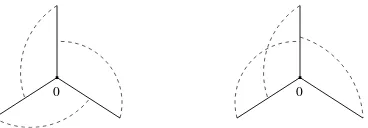
A laceL on a star shapeS of degree 1 (or equivalently 2) is necessarily minimal by Definitions 2.3 and 2.1. For a lace on a star shape of degree 3 this need not be true. See Figure 9 for an example of a minimal and a non-minimal lace for ∆ = 3. A non-minimal lace contains a bond
st that is “removable” in the sense that L\ {st} is still a lace. In general such a bond is not unique. One can easily construct a lace on a star shaped network of degree 3 for which each of the bondss1t1, . . . , s3t3 covering the branch point satisfyL\ {siti} ∈ L(S).
Definition 2.8 (Acyclic). A lace L on S3 is acyclicif there is at least one branch S
e (called a
specialbranch) such that there is exactly one bond,stin L, covering the branch point ofS3 that
b b b
b b
Figure 8: An illustration of the construction of a lace from a connected graph. The first figure shows a connected graph Γ on a starS(3n1,n2,n3). The intermediate figures show each of theLΓ(e)
fore∈Fb, while the last figure shows the laceLΓ.
0 0
0 0
Figure 10: Basic examples of a cyclic and an acyclic lace.
It is obvious that in the above definition,stis the bond inLassociated to branchSe. In addition,
it is immediate from Definition 2.8 that for a cyclic lace, the bonds covering the branch point can be ordered as {sktk :k= 1, . . . ,3}, with tk and sk+1 on the same branch for each k (with
s4 identified with s1). See Figure 10 for an example of this classification.
Let Le,N(S) be the set of laces L∈ LN(S), such thatL\ {sete} ∈ LN−1(S), where sete is the
bond inL associated to Se. Let
Lmine,N−1 ={L∈ LminN−1(S) :∃stwith L∪ {st} ∈ Le,N(S), stassociated to Se forL∪ {st}}, (2.3)
and observe that Le,Nmin−1 is a subset of the (acyclic) laces with two bonds covering the branch point. GivenL∈ Le,Nmin−1, define
Pe(L) ={st:L∪ {st} ∈ Le,N(S), stassociated to Se forL∪ {st}}. (2.4)
Using∪• to denote a disjoint union, as shown in [19],
Le,N(S)⊆∪•L
∈Le,Nmin−1(S) •
∪st∈Pe(L){L∪ {st}}. (2.5)
The set Pe(L) can be totally ordered firstly according to distances from the branch point and
then by branch numbers. The following Lemma is proved in [19].
Lemma 2.9 ([19], Lemma 6.4). Given a laceL∈ Lmine,N−1 and st∈ Pe(L),
C(L∪ {st}) =C(L)∪ {• ij ∈ Pe(L) :ij < st}. (2.6)
2.3 The Expansion
Here we examine products of the formQst∈EN[1 +Ust]. Following the method of [20], we write
Y
st∈EN
[1 +Ust] =
Y
st∈EN\R
[1 +Ust]−
Y
st∈EN\R
[1 +Ust]
Ã
1− Y
st∈R
[1 +Ust]
!
. (2.7)
Define K(M) = Qst∈EM\R[1 +Ust]. Expanding this we obtain, for each possible subset of
EM\ R, a product ofUst forstin that subset. The subsets ofEM\ Rare precisely the graphs
on Mwhich contain no elements ofR, hence
K(M) = X
Γ∈GM−R
Y
st∈Γ
where the empty product Qst∈∅Ust = 1 by convention. Similarly we define
stin that subset.
In Section 4 we will haveUst ∈ {−1,0}whence
We use (2.5) and (2.6) to bound the contribution to (2.11) from non-minimal laces (containing
N ≥3 bonds) as follows,
Now using the fact (e.g. see [19]) that
0≤ X
the last line of (2.12) is bounded by
2.3.1 Recursion type expression for K(N)
Recall thatN =N(α, ~n) whereα∈Σr and~n∈N2r−3, for somer≥2. Ifr= 2 then letbbe the
root ofN. Otherwise letbbe the branch point neighbouring the root ofN. In each case letSN−
be the largest connected subnetwork ofN containingband no vertices that are adjacent to any other branch points of N (SN− could be empty or a single vertex). Observe that for any graph Γ∈ GN−R\ Eb
N, the subnetworkAb(Γ) contains no branch point ofN other thanb (ifr≥3) and
hence is a star shape of degree 0, 1 or 3.
Definition 2.10. If M is a connected subnetwork of N then we define N \ M to be the set of vertices of N that are not in M together with the edges of N connecting them. In general (N \ M)∪ M contains fewer edges than N, and N \ M need not be connected. However if
M ⊂ SN− then N \ M has at most 3 connected components (at most 1 if r = 2) and we write (N \ M)i,i= 1,2,3 for these components, where we allow(N \ M)i =∅.
Definition 2.10 allows us to write
K(N) = X
Γ∈GN−R\ENb
Y
st∈Γ
Ust+
X
Γ∈Eb N
Y
st∈Γ
Ust
= X
A⊂SN−:
b∈A
X
Γ∈Gcon A
Y
st∈Γ
Ust
3
Y
i=1
X
Γi∈G(−RN \A)i
Y
siti∈Γ i
Usiti+
X
Γ∈Eb N
Y
st∈Γ
Ust,
(2.14)
where the sum over A is a sum over connected subnetworks of N containing b and no vertices adjacent to any other branch points ofN. Some of the (N \ A)i may be a single vertex or empty
and we definePΓi∈G∅Qsiti∈Γ
iUsiti = 1. Defining E
(b)(N) =P Γ∈Eb
N
Q
st∈ΓUst, we have
K(N) = X
A⊂SN−:
b∈A
J(A)
3
Y
i=1
K((N \ A)i) +E(b)(N). (2.15)
Depending onN, the first term of (2.15) may be zero sinceSN− may be empty. The fact that for any A contributing to this first term, the subtrees (N \ A)i are of degree ri < r is what allows
for an inductive proof of Theorem 1.14.
Ifr= 2 thenN contains no branch point. In this case we may identify the star-shaped network
S1(m) with the interval [0, m] and (2.14)-(2.15) reduce to
K([0, n]) = X
m≤n
J([0, m])K([m+ 1, n]), (2.16)
which is the usual relation for the expansion ofK(·) on an interval for this notion of connectivity (see for example [8]). Otherwisebis a branch point ofN and we letK(∅)≡1, andIi =Ii(N) be
the indicator function that the branchiis incident tob and another branch pointbi. Therefore
for a fixed networkN such thatSN− is nonempty,ni−2I2 =ni−2I2(N) is equal to eithern2−2
(if branch 2 is incident to band another branch point bi) orni. Then (2.14)-(2.15) give
K(N) = X
m1≤n1
X
m2≤n2−2I2 m3≤n3−2I3
J(Sm~)
3
Y
i=1
whereSm~ is a star-shaped network satisfying
Sm~ =
{b} ifm~ =~0,
S3
~
m ifmi 6= 0 for alli,
S[0, mi] ifmi 6= 0 andmj = 0 forj6=i,
S[−mj, mi] ifj > i, mj 6= 0, mi6= 0, andmk= 0 fork6=i, j.
(2.18)
In the case where there is another branch point be that is adjacent to b in N (so that n2 or
n3 is 1), the sum over at least one of m2, m3 in (2.17) is empty. However note that this case
contributes to the termE(b)(N), as required.
3
The 2-point function
In this section we prove Theorem 1.12 using an extension of the inductive approach to the lace expansion of [17]. The extension of the induction approach is described and proved in a general setting in [15]. Broadly speaking there are two main ingredients involved in applying the results of [15]. Firstly we must obtain a recursion relation for the quantity of interest, the Fourier transform of the 2-point function, and massage this relation so that it takes the form (1.6), with each fi,gi having continuous second derivative in a neighbourhood of 0 and f0(k;z) = 1,
f1(k;z) = zDb(k), e1(k;z) = 0. Secondly we must verify the hypotheses that certain bounds
on the quantities fm for 1≤m ≤n appearing in (1.6) imply further bounds on the quantities
gm, em, for 2≤m ≤n+ 1. This second ingredient consists of reducing the bounds required to
diagrammatic estimates, and then estimating the relevant diagrams.
In Section 3.1 we prove a recursion relation of the form (1.6) for a quantity closely related to the Fourier transform of the 2-point function. In Section 3.2 we state the assumptions of the inductive approach for a specific choice of parameters corresponding to our particular model. In Section 3.3 we reduce the verification of these assumptions to proving a single result, Proposition 3.6. Assuming Proposition 3.6, the induction approach then yields Theorem 3.7, which we show in Section 3.4 implies Theorem 1.12. The diagrammatic estimates involved in proving Proposition 3.6 provide the most model dependent aspect of the analysis and these are postponed until Section 5.
3.1 Recursion relation for the 2-point function
Recall Definitions 1.4, 1.6, and 1.8. Also recall from Definition 1.10 that the two point function is defined as
tn(x;ζ) =ζn
X
T∈Tn(x)
W(T).
Now T ∈ Tn(x) if and only if T is the union (as a set of vertices and edges) of an n-step
(self-avoiding) walk ω from o to x together with a collection of mutually avoiding branches
Ri ∈ T(ω(i)), i= 0,1, . . . , n(see Figure 11). Let
Ust =U(Rs, Rt) =
½
−1, ifRs∩Rt6=∅
0
x
0
x
0
x
Figure 11: The first figure is of a lattice tree T ∈ Tn(x) for n = 17. The second figure shows
the backboneω, while the third shows the mutually avoiding lattice treesR0, . . . , Rn emanating
from the backbone.
ThenQ0≤s<t≤n[1 +Ust] is the indicator function that all theRi avoid each other. Summarising
the above discussion and using the fact that the weight W(T) of a tree factorises into (bond) disjoint components (see Definition 1.7) we can write,
tn(x;ζ) =ζn
X
ω:o→x,
|ω|=n
W(ω) X
R0∈T(ω(0))
W(R0)
X
R1∈T(ω(1))
W(R1)· · ·
X
Rn∈T(ω(n))
W(Rn)
Y
0≤s<t≤n
[1 +Ust],
(3.2)
where the first sum is overrandom walk pathsof lengthnfrom 0 tox. To simplify this expression, we abuse notation and replace (3.2) with
tn(x;ζ) =ζn
X
ω:o→x,
|ω|=n
W(ω)
n
Y
i=0
X
Ri∈T(ω(i))
W(Ri)
Y
0≤s<t≤n
[1 +Ust]. (3.3)
Recall Definition 2.1 and the discussion following it. The set of vertices [0, n] corresponds to the set of vertices of N(α, n), where α is the unique shape in Σ2. Since this N contains no branch
points, we have R =∅ and therefore from Section 2.3 we have Q0≤s<t≤n[1 +Ust] = K(N) =
K([0, n]). Hence
tn(x;ζ) =ζn
X
ω:o→x
|ω|=n
W(ω)
n
Y
i=0
X
Ri∈T(ω(i))
W(Ri)K([0, n]). (3.4)
Definition 3.1. For m≥0 we define
πm(x;ζ) =ζm
X
ω:o→x
|ω|=m
W(ω)
m
Y
i=0
X
Ri∈T(ω(i))
W(Ri)J([0, m]). (3.5)
Note that for m= 0 this is simply PR0∈T(0)W(Ri) =ρ(o), if x= 0, and zero otherwise.
Definition 3.2. The convolution of functions fi, i= 1, . . . n is defined as the function
(f1∗f2∗ · · · ∗fn)(x) =
X
y1∈Zd
X
y2∈Zd
· · · X
yn−1∈Zd
f1(y1)
nY−1
i=2
at all points x where this converges.
We often write f(n)(x) for the n-fold convolution convolution of f with itself, e.g. f(2)(x) = (f ∗f)(x).
The following recursion relation is the starting point for obtaining a relation of the form (1.6).
Proposition 3.3. For x∈Zd,
tn+1(x;ζ) =
n
X
m=1
(πm∗ζpcD∗tn−m)(x;ζ) +πn+1(x;ζ) +ρ(o)(ζpcD∗tn)(x;ζ). (3.6)
Proof. Firstly recall thattnandDhave finite range. Similarly, the bound (2.11) and the fact that
there are only finitely many laces on S([0, n]) for each nshows that |πm(x;ζ)| ≤cmζmD(m)(x)
for some cn depending on n but not x. In particular each πm(x;ζ) also has finite range and
therefore all of the convolutions in (3.6) exist for all x. By definition
tn+1(x;ζ) =ζn+1
X
ω:o→x,
|ω|=n+1
W(ω)
nY+1
i=0
X
Ri∈T(ω(i))
W(Ri)K([0, n+ 1]). (3.7)
Equation (2.16) gives
K([0, n+ 1]) =K([1, n+ 1]) +
n
X
m=1
J([0, m])K([m+ 1, n+ 1]) +J([0, n+ 1]). (3.8)
Putting this expression into equation (3.7) gives rise to three terms which we consider separately.
1. The contribution from graphs for which 0 is not covered by any bond: We break the backbone from 0 to x (a walk of length n+ 1) into a single step walk and the remaining
n-step walk as follows.
ζn+1 X
ω:o→x,
|ω|=n+1
W(ω)
nY+1
i=0
X
Ri∈T(ω(i))
W(Ri)K[1, n+ 1]
= X
R0∈T(o)
W(R0)
X
y∈ΩD
X
ω1:o→y,
|ω1|=1
ζW(ω1)
X
ω2:y→x,
|ω2|=n
ζnW(ω2)
nY+1
i=1
X
Ri∈T(ω2(i−1))
W(Ri)K([1, n+ 1]),
(3.9)
whereK[1, n+ 1] depends on R1, . . . , Rn+1 but notR0. Therefore using the substitutions
R′j =Rj+1 this is equal to
ρ(o) X
y∈ΩD
X
ω1:o→y,
|ω1|=1
ζW(ω1)
X
ω2:y→x,
|ω2|=n
ζnW(ω2)
n
Y
j=0
X
R′j∈T(ω
2(j))
W(R′j)K([0, n])
=ρ(o) X
y∈ΩD
pcζD(y)tn(x−y;ζ) =ρ(o)pcζ(D∗tn)(x).
2. The contribution from graphs which are connected on [0, n+ 1]: 1 andn−m respectively
ζn+1 X
Dividing both sides of (3.6) by ρ(o) and taking Fourier transforms, we get
2) f0(k;z) = 1, f1(k;z) =g1(k;z) =zDb(k), ande1(k;z) = 0.
3) Forn≥2,
fn(k;z) =
btn(k;ζ)
ρ(o) , gn(k;z) =
b
πn−1(k;ζ)
ρ(o) zDb(k)
en(k;z) =gn−1(k;z)
"
bt1(k;ζ)
ρ(o) −zDb(k)
#
+πbn(k;ζ)
ρ(o) .
(3.15)
We note from (3.14) withn= 0 that sincet0(x) =ρ(o)Ix=0, we havebt0(k) =ρ(o) and
b
t1(k;ζ)
ρ(o) −zDb(k) =
b
π1(k;ζ)
ρ(o) . (3.16)
Therefore forn≥2
en(k;z) =gn−1(k;z)bπ1(k;ζ)
ρ(o) +
b
πn(k;ζ)
ρ(o) . (3.17)
Forn≥3 this is
en(k;z) = b
πn−2(k;ζ)
ρ(o) zDb(k)
b
π1(k;ζ)
ρ(o) +
b
πn(k;ζ)
ρ(o) .
Lemma 3.5. The choices of fm, gm, em above satisfy (1.6).
Proof. This is an easy exercise using (3.14).
3.2 Assumptions of the induction method
The induction approach to the lace expansion of [17] is extended in [15] with the introduction of two parameters θ and p∗ and a set B ⊂[1, p∗]. In this section we apply the extension with the choicesθ= d−24,p∗ = 2, B ={2}and we define β =L−pd∗ =L−d2. We have already shown
in Section 3.1 that for our choices of fm, gm, em as given in Definition 3.4,
fn+1(k;z) =
n+1
X
m=1
gm(k;z)fn+1−m(k;z) +en+1(k;z) (n≥0),
withf0(k;z) = 1. The assumptions of [15] in our lattice trees setting are as follows.
Assumption S. For every n ∈ N and z > 0, the mapping k 7→ fn(k;z) is symmetric under
replacement of any componentki ofkby −ki, and under permutations of the components of k.
The same holds foren(·;z) andgn(·;z). In addition, for eachn,|fn(k;z)|is bounded uniformly
ink∈[−π, π]d andz in a neighbourhood of 1 (which may depend on n). The functionsf n and
gn have continuous second derivatives with respect tokin a neighbourhood of 0 for everyn.
Assumption D. As part of Assumption D, we assume that:
(i) Dis normalised so that ˆD(0) = 1, and has 2 + 2ǫmoments for some ǫ∈(0,1∧d−8 2 ), i.e.,
X
x∈Zd
(ii) There is a constantC such that, for allL≥1,
kDk∞≤CL−d, σ2=σL2 ≤CL2, (3.19)
(iii) Definea(k) = 1−Dˆ(k). There exist constants η, c1, c2 >0 such that
c1L2|k|2≤a(k)≤c2L2|k|2 (kkk∞≤L−1), (3.20)
a(k)> η (kkk∞≥L−1), (3.21)
a(k)<2−η (k∈[−π, π]d). (3.22)
Forh: [−π, π]d→C, we define
∇2h(k0) =
d
X
j=1
∂2 ∂k2
j
h(k)
k=k0
. (3.23)
The relevant bounds onfm, which a priori may or may not be satisfied, are that
kDb2fm(·;z)k2 ≤
K
Ld2m
d
4
, |fm(0;z)| ≤K, |∇2fm(0;z)| ≤Kσ2m, (3.24)
for some positive constantK. Recall that
β =L−d2. (3.25)
Assumption E. There is an intervalI ⊂[1−α,1+α] withα∈(0,1), and a functionK 7→Ce(K),
such that: if (3.24) holds for some K, L≥1,z∈I and all m with 1≤m ≤n, then for this K,
Land z, and for allk∈[−π, π]d and 2≤m≤n+ 1, the following bounds hold:
|em(k;z)| ≤Ce(K)βm−
d−4
2 , |em(k;z)−em(0;z)| ≤Ce(K)a(k)βm−
d−6 2 .
Assumption G. There is an interval I ⊂[1−α,1 +α] withα ∈(0,1), and a function K 7→ Cg(K), such that: if (3.24) holds for some K, L≥1,z∈I and all m with 1≤m≤n, then for
this K,Land z, and for all k∈[−π, π]d and 2≤m≤n+ 1, the following bounds hold:
|gm(k;z)| ≤Cg(K)βm−
d−4
2 , |∇2gm(0;z)| ≤Cg(K)σ2βm−
d−6 2 ,
|∂zgm(0;z)| ≤Cg(K)βm−
d−6 2 ,
|gm(k;z)−gm(0;z)−a(k)σ−2∇2gm(0;z)| ≤Cg(K)βa(k)1+ǫ
′
m−d−26+ǫ′,
3.3 Verifying assumptions
Assumption S: The quantities fn(k;z), n = 0,1, . . . are (up to constants) the Fourier
trans-forms of tn(x, ζ), and hence have all required symmetries since Db does. Similarly the πm are
symmetric, so that the quantitiesgn, en also have the required symmetries. Nowf0= 1 is
triv-ially uniformly bounded ink and z≤2. Recall that Pxtn(x;ζ)≤(ζpc)nρ(o)n+1PxD(n)(x) =
(ζpc)nρ(o)n+1, where D(n) denotes the n-fold convolution of D. Then for n ≥ 1, |fn(k, z)| ≤
ρ(o)−1Pxtn(x;ζ) ≤(ζpcρ(o))n=zn so that fn is bounded uniformly in k∈[−π, π]d and z in
an n-dependent neighbourhood of 1. Continuity of the second derivatives holds for each n as the quantities in question are Fourier transforms of functions with finite support. An immediate consequence of Assumption S is that the mixed partials of fn and gn atk = 0 are all equal to
zero.
Assumption D: By Definition 1.4 and Remark 1.5, (3.18) and (3.19) hold trivially. The remaining conditions (iii) are verified in [17].
We therefore turn our attention to verifying assumptions E and G. Recall from Definition 3.4 and (3.17) that forn≥2,gnandencould be expressed in terms of the quantitiesπbmform≤n.
In Section 5 we will prove the following proposition.
Proposition 3.6 (πm bounds). For every K ≥ 1 there exists Lπ(K) ≥1 such that: if (3.24) holds for all L ≥ L0, and m ≤ n with this K, for some L0 ≥Lπ and z ∈ (0,2), then for this
K, z and each L≥L0, m≤n+ 1and q∈ {0,1,2},
X
x
|x|2q|πm(x;ζ)| ≤
C(K)σ2qβ2−6ν d
md−24−q
, (3.26)
where ζ =ρ(o)−1p−c1z, the constant C =C(K, d) does not depend onL, m andz, andν >0 is the constant appearing in Theorem 1.9.
We chooseν <1 in (1.4) so that 2−6ν
d >1 and thereforeβ2− 6ν
d ≤β =L− d
2. We now direct our
efforts towards verifying assumptions E and G, in the case where the conditions in Proposition 3.6 are met.
Assumption E: Suppose that there exist K ≥1, L0 ≥Lπ(K) andz ∈(0,2) such that (3.24)
holds for this K, z and all L ≥ L0 and 1 ≤ m ≤ n. Fix such an L. Since L0 ≥ Lπ(K),
Proposition 3.6 holds forL≥L0. Recall that e1(k;z) = 0 and observe from (3.17) that
|e2(k;z)|=
¯ ¯ ¯
¯zDb(k)b
π1(k;ζ)
ρ(o) +
b
π2(k;ζ)
ρ(o)
¯ ¯ ¯ ¯≤z
¯ ¯ ¯ ¯b
π1(k;ζ)
ρ(o)
¯ ¯ ¯ ¯+
¯ ¯ ¯ ¯b
π2(k;ζ)
ρ(o)
¯ ¯ ¯ ¯≤
C′(K)β2−6dν
2d−24
, (3.27)
where we have applied Proposition 3.6 with |bπm(k;ζ)| ≤ Px|πm(x;ζ)|, and have also used
ρ(o)≥1. Similarly for 3≤m≤n+ 1,
|em(k;z)|=
¯ ¯ ¯
¯bπm−2(k;ζ)zDb(k)b
π1(k;ζ)
ρ(o)2
¯ ¯ ¯ ¯+
¯ ¯ ¯ ¯b
πm(k;ζ)
ρ(o)
¯ ¯ ¯ ¯
≤ C(K)β 2−6ν
d
ρ(o)2(m−2)d−24
zC(K)β2−6dν +C(K)β 2−6ν
d
ρ(o)md−24
≤ C′(K)β 2−6ν
d
md−24
.
Thus we have obtained the first bound of Assumption E. It follows immediately that for all
the method of [19].
Leth:Zd→Rbe finitely supported and symmetric in each coordinate and under permutations of coordinates. Thenbh(k) =Pxcos(k·x)h(x) and
In particular choosingη= 0 we get
Form≥3, recall that gm−1(k;z) = bπm−ρ(2o()k;ζ)zDb(k) which gives
which gives the first bound of Assumption G.
For the second bound we note that by symmetry the first derivatives of bπm and Db vanish at 0.
Hence form≥2,
This verifies the second bound of Assumption G. Next form≥2, we have that
which proves the third part of assumption G.
sincea(k)> η, and where the constant depends onη. This satisfies the final part of assumption G forkkk∞≥L−1.
For kkk∞ ≤ L−1, we again use the method of [19]. By the triangle inequality we bound |gm(k;z)−gm(0;z)−a(k)σ−2∇2gm(0;z)|by
¯ ¯ ¯
¯gm(k;z)−gm(0;z)−|
k|2
2d ∇
2g
m(0;z)
¯ ¯ ¯ ¯+
¯ ¯ ¯
¯(a(k)−a(0))σ−2−|
k|2
2d
¯ ¯ ¯
¯|∇2gm(0;z)|. (3.40)
Recall that form ≥ 2, gm(k;z) = ρ(zo)(π\m∗D)(k). On the first term we apply the analysis of
the first term of (3.29), to the symmetric function πm−1∗D. Choosing η =ǫ′ we see that the
first term of (3.40) is bounded by
zC|k|2+2ǫ′X
x
|x|2+2ǫ′|(πm−1∗D)(x)|, (3.41)
with the constant independent ofǫ′. By H¨older’s inequality
X
x
|x|2+2ǫ′|(πm−1∗D)(x)| ≤
à X
x
|(πm−1∗D)(x)|
!1−ǫ′
2 ÃX
x
|x|4|(πm−1∗D)(x)|
!1+ǫ′
2
. (3.42)
Applying Proposition 3.6 withq = 0 gives
X
x
|(πm−1∗D)(x)| ≤
X
y
|πm−1(y)|
X
x
D(x−y)≤ C(K)β 2−6ν
d
md−24
. (3.43)
We now apply Proposition 3.6 withq = 0,2 together with the inequality (a+b)4 ≤8(a4+b4) to get
X
x
|x|4|(πm−1∗D)(x)| ≤8
à X
y
|y|4|πm−1(y)|
X
x
D(x−y) +X
y
|πm−1(y)|
X
x
|x−y|4D(x−y)
!
≤C
à X
y
|y|4|πm−1(y)|+
X
y
|πm−1(y)|σ4
!
≤σ
4C′(K)β2−6ν d
md−28
.
(3.44)
Note that we have used Remark 1.5 to obtainPx|x|rD(x)≤Cσrwith the constant independent
ofL (it may depend on r). Putting (3.43) and (3.44) back into (3.42) we get
X
x
|x|2+2ǫ′|πm−1(x)| ≤
Ã
C(K)β2−6dν
md−24
!1−ǫ′
2 Ã
σ4C(K)β2−6ν d
md−28
!1+ǫ′
2
≤ σ
2(1+ǫ′)C(K)β2−6ν d
md−26−ǫ′
.
Combining (3.45) with (3.41) gives
It remains to verify this bound for the term inside the second absolute value in expression (3.40). For this term we write
¯
and proceed as for the first term to obtain
¯
Together with Proposition 3.6 withq = 1 this gives
¯
We have now verified that Assumptions S,D,E,G all hold, provided L≥Lπ, i.e. assuming that
Proposition 3.6 holds. Thus assuming Proposition 3.6, we may apply the induction method of [15] and obtain the following theorem.
(d) The constants zc, A′ and v are all 1 +O
In particular, provided Proposition 3.6 holds, the induction method shows that there exists
L0, K ≥ 1 such that (3.24) holds for all m and all L ≥L0 for this K. The induction method
itself is rather complicated but is logically structured as follows: Firstly we find the functions
Ce and Cg in Assumptions E and G, as appears in the verification of these assumptions for
large L above. The induction method then defines a host of constants including K, that are independent of L, but depend on the functions Ce, Cg. It also identifies Lind ≫ 1, depending
on these constants, for which it is required that L≥Lind to advance (3.24). One then chooses
L0 =Lπ∨Lind, so that Proposition 3.6 holds and the advancement of (3.24) for allL≥L0 for
our chosenK.
3.4 Proof of Theorem 1.12
In this section we show that Theorem 1.12 follows from Theorem 3.7(a). Comparing the two theorems and settingA=A′ρ(o) (recall thatζc =zcρ(o)−1p−c1), it is clear that to prove Theorem
1.12 it is sufficient to prove the following two lemmas. The first incorporates the continuous time variabletinto the asymptotic formula (3.48), while the second confirms that our artificially introduced parameterζ is trivial.
Lemma 3.8. Ford, γ, δ and L0 as in Theorem 3.7, there exists a constant C0 =C0(d, γ)>0
where the error estimate is uniform in
We leave it as an exercise to show that there exists a constant C0 such that {k : |k|2 ≤
C0t−1log(⌊nt⌋)} ⊂ Hn,t, and thus (3.50) holds with the error estimate uniform in {k :|k|2 ≤
C0log(⌊nt⌋)}. Since⌊nt⌋ ≤ntin the first error term of (3.50), and
¯ ¯ ¯ ¯e−
|k|2⌊nt⌋
2dn −e− |k|2t
2d
¯ ¯ ¯ ¯≤ |
k|2
2d
µ
t−⌊nt⌋ n
=O
µ
|k|2
n
,
we have proved Lemma 3.8.
Proof of Lemma 3.9. The susceptibility,χ(z) is
χ(z)≡X
n
fn(0;z) =
X
n
btn(0;ζ)
ρ(o) =
X
n
ζn 1 ρ(o)
X
x
X
T∈Tn(x)
W(T)≡χ¯(ζ), (3.51)
whereζ =zρ(o)−1p−c1. By Theorem 3.7 there exists aζc such that
ζcn 1 ρ(o)
X
x
X
T∈Tn(x)
W(T)→A >0, (3.52)
so that
1
ρ(o)
X
x
X
T∈Tn(x)
W(T)
1
n → 1
ζc
.
Thus the radius of convergence of ¯χ(ζ) is ζc > 0. Since P|x|<M(|x| ∨1)a−d ≃ Ma, it follows
from Theorem 1.9 that ¯χ(1) =∞ which implies that ζc ≤1.
Forζ <1, Pnζntn(x)≤e−c(ζ)|x|ρ(x), which implies that
X
x
ζntn(x)≤(
p
ζ)nX
x
X
m≥n
(pζ)mtm(x)≤(
p
ζ)nX
x
e−c′(ζ)|x|ρ(x), (3.53)
which goes to 0 asn→ ∞. Henceζc≥1 and the result follows.
Assuming that Proposition 3.6 holds, we have now verified Lemmas 3.8 and 3.9, and hence we have proved Theorem 1.12. We postpone the proof of Proposition 3.6 to Section 5.
4
The
r
-point functions
4.1 Preliminaries
Recall from Definitions 1.3 and 1.13 that for fixedr≥2,˜n∈Z+r−1 andx˜∈Rd(r−1), we have
Tn˜(˜x) ={T ∈ T(o) :xi∈Tni, i= 1, . . . , r−1}
and
tr˜n(˜x) =
X
T∈T˜n(˜x)
W(T),
where we may have xi = xj and ni = nj for some i 6= j. For T ∈ T(o, x), let TÃx be the
backbone inT from 0 to x.
Definition 4.1 (Bare tree). For n˜ ∈ Zr+−1 and x˜ ∈ Zd+(r−1), a lattice tree B is said to be an (n˜,˜x) bare tree if B ∈ Tn˜(˜x) and ∪ri=1−1BÃxi =B. We let B(˜n,˜x) denote the set of (n˜,˜x) bare trees. If B ∈ B(˜n,˜x) then we write TB = {T ∈ T(o) : B ⊆ T} for the set of lattice trees containing B as a subtree.
Since everyT ∈ Tn˜(x˜) has a unique minimal connected subtree (∪ir=1−1TÃxi) connecting 0 to the
xi,i= 1, . . . , r−1, we have
tr˜n(˜x) =
X
B∈B(n˜,˜x)
X
T∈TB
W(T). (4.1)
Thedegreeof a vertexx∈B is the number of bonds{a, b} ∈B such that either a=x orb=x.
Definition 4.2 (Branch point). Let B ∈ B(˜n,x˜). A vertex x ∈ B is a branch point of B if there exist i6=j such thatxi 6=o and xj 6=o are distinct leaves (vertices of degree 1) of B and
BÃxi∩BÃxj =BÃx.
As they are defined in terms of the leaves of B ∈ B(˜n,˜x), branch points of B depend on B
but not the setB(n˜,˜x) of whichB is a member. In particular if B is also inB(˜n′,x˜′) then our definition gives rise to the same set of branch points. By definition, a branch point that is not the origin must have degree ≥3. It is clear that the number of leaves6=ois at least 1 plus the number of branch points, so ifB ∈B(n˜,˜x) forx˜∈Zd(r−1)thenB contains at mostr−2 branch
points.
Definition 4.3 (Degenerate bare tree). For fixed r ≥ 3, ˜n ∈ Z+r−1 and ˜x ∈ Rd(r−1), a bare
treeB ∈B(n˜,˜x) is said to benon-degenerate if B contains exactlyr−2 distinct branch points, each of degree 3, none of which is the origin. Otherwise B is said to be degenerate. We write
BD(n˜,˜x) for the set of degenerate trees in B(˜n,˜x) and set BcD(n˜,˜x) =B(˜n,˜x)\BD(˜n,x˜).
Clearly from (4.1) we have
tr˜n(˜x) =
X
B∈Bc
D(n˜,˜x)
X
T∈TB
W(T) + X
B∈BD(n˜,˜x)
X
T∈TB
W(T). (4.2)
Definition 4.4. Let B∈B(˜n,x˜). Two distinct verticesy,y∗ inB are said to benet-neighbours inB if the unique path in B from y to y∗ contains no branch points of B other than (perhaps)