El e c t ro n ic
Jo ur n
a l o
f P
r o b
a b i l i t y
Vol. 13 (2008), Paper no. 56, pages 1624–1671.
Journal URL
http://www.math.washington.edu/~ejpecp/
Some families of increasing planar maps
Marie Albenque LIAFA, CNRS UMR 7089 Universit´e Paris Diderot - Paris 7
75205 Paris Cedex 13 [email protected]
Jean-Fran¸cois Marckert∗
CNRS, LaBRI, UMR 5800 Universit´e Bordeaux 1 351 cours de la Lib´eration
33405 Talence cedex [email protected]
Abstract
Stack-triangulations appear as natural objects when one wants to define some families of increasing triangulations by successive additions of faces. We investigate the asymptotic behavior of rooted stack-triangulations with 2nfaces under two different distributions. We show that the uniform distribution on this set of maps converges, for a topology of local convergence, to a distribution on the set of infinite maps. In the other hand, we show that rescaled byn1/2
, they converge for the Gromov-Hausdorff topology on metric spaces to the continuum random tree introduced by Aldous. Under a distribution induced by a natural random construction, the distance between random points rescaled by (6/11) lognconverge to 1 in probability.
We obtain similar asymptotic results for a family of increasing quadrangulations.
Key words: stackmaps, triangulations, Gromov-Hausdorff convergence, continuum random tree.
AMS 2000 Subject Classification: Primary 60C05, 60F17.
Submitted to EJP on December, 2007, final version accepted Auguest 25, 2008.
∗
1
Introduction
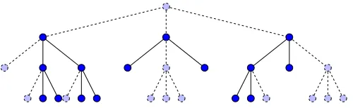
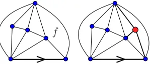
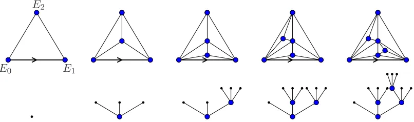
Consider a rooted triangulation of the plane. Choose a finite triangular face ABC and add inside a new vertex O and the three edges AO, BO and CO. Starting at time 1 from a single rooted triangle, afterksuch evolutions, a triangulation with 2k+ 2 faces is obtained. The set of triangulations △2k with 2k faces that can be reached by this growing procedure is not the set of all rooted triangulations with 2k faces. The set △2k – called the set of stack-triangulations with 2k faces – can be naturally endowed with two very different probability distributions:
- the first one, very natural for the combinatorial point of view, is the uniform distribution
U△2k,
- the second probability Q△2k maybe more realistic following the description given above, is the probability induced by the construction when the faces where the insertion of edges are done are chosen uniformly among the existing finite faces.
Figure 1: Iterative construction of a stack-triangulation. Note that three different histories lead to the final triangulation.
The aim of this paper is to study these models of random maps. Particularly, we are interested in large maps when the number of faces tends to +∞. It turns out that this model of triangulations is combinatorially simpler that the set of all triangulations. Under the two probabilitiesQ△2kand
U△
2k we exhibit a global limit behaviorof these maps.
A model of increasing quadrangulations is also treated at the end of the paper. In few words this model is as follows. Begin with the rooted square and successively choose a finite face ABCD, add inside a node O and two new edges: AO and OC (or BO and OD). When these two choices of pair of edges are allowed we get a model of quadrangulations that we were unable to treat as wanted (see Section 8.1). When only a suitable choice is possible, we get a model very similar to that of stack-triangulations that may be endowed also with two different natural probabilities. The results obtained are, up to the normalizing constants, the same as those obtained for stack-triangulations. For sake of briefness, only the case of stack-triangulations is treated in details.
We present below the content of the paper and a rough description of the results, the formal statements being given all along the paper.
1.1 Contents
In Section 2 we define formally the set of triangulations△2n and the two probabilitiesU△2n and
3n−2 nodes deeply used in the paper. In Section 3 are presented the two topologies considered in the paper:
- the first one is an ultra-metric topology called topology of local convergence. It aims to describe the limiting local behavior of a sequence of maps (or trees) around their roots,
- the second topology considered is the Gromov-Hausdorff topology on the set of compact metric spaces. It aims to describe the limiting behavior of maps (or trees) seen as metric spaces where the distance is the graph distance. The idea here is to normalize the distance in maps by the order of the diameter in order to observe a limiting behavior.
In Section 4.1 are recalled some facts concerning Galton-Watson trees conditioned by the sizen, when the offspring distribution isνter= 13δ3+23δ0 (the tree is ternary in this case). It is recalled
(Section 4.2) that they converge under the topology of local convergence to an infinite branch, (the spine or infinite line of descent) on which are grafted some critical ternary Galton-Watson trees; rescaled by n1/2 they converge for the Gromov-Hausdorff topology to the continuum random tree (CRT), introduced by Aldous [1] (Section 5.1).
Sections 4 and 5 are devoted to the statements and the proofs of the main results of the paper concerning random triangulations underU△2n, whenn→+∞. The strongest theorems of these parts, that may also be considered as the strongest results of the entire paper, are:
- the weak convergence of U△
2nfor the topology of local convergence to a measure on infinite triangulations (Theorem 12, Section 4),
- the convergence in distribution of the metric of stack-triangulations for the Gromov-Hausdorff topology (the distance being the graph distance divided by√6n/11) to the CRT (Theorem 15, Section 5). It is up to our knowledge, the only case where the convergence of the metric of a model of random maps is proved (apart from trees).
Section 7 is devoted to the study of △2n under Q△2n. Under this distribution, there is no local convergence around the root, its degree going a.s. to +∞. Theorem 21 says that seen as metric spaces they converge normalized by (6/11) logn, in the sense of the finite dimensional distributions, to the discrete distance on [0,1] (the distance between different points is 1). Hence, there is no weak convergence for the Gromov-Hausdorff topology, the space [0,1] under the discrete distance being not compact. Section 7.2 contains some elements stating the speed of growing of the maps (the evolution of the node degrees, or the size of a sub-map).
Section 8 is devoted to the study of a model of quadrangulations very similar to that of stack-triangulations, and to some questions related to another family of growing quadrangulations. Last, the Appendix, Section 9, contains the proofs that have been extracted from the text for sake of clarity.
1.2 Literature about stack-triangulations
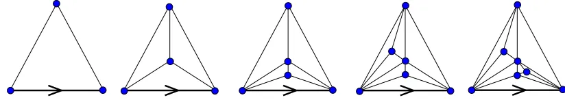
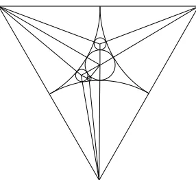
Stack-triangulations appear in the literature for very various reasons. In Bernardi and Bonichon [7], stack-triangulations are shown to be in bijection with intervals in the Kreweras lattice (and realizers being both minimal and maximal). The set of stack triangulations coincides also with the set of plane triangulations having a unique Schnyder wood (see Felsner and Zickfeld [21]). These triangulations appear also around the problem of graph uniquely 4-colorable. A graph G is uniquely 4-colorable if it can be colored with 4 colors, and if every 4-coloring of G produces the same partition of the vertex set into 4 color classes. There is an old conjecture saying that the family of maps having this property is the set of stack-triangulations. We send the interested reader to B¨ohme & al. [10] and references therein for more information on the question. As illustrated on Figure 2, these triangulations appear also in relation with Apollonian circles. We refer to Graham & al. [25], and to several other works of the same authors, for remarkable properties of these circles.
The so-called Apollonian networks, are obtained from Apollonian space-filling circles packing. First, we consider the Apollonian space-filling circles packing. Start with three adjacent circles as on Figure 2. The hole between them is filled by the unique circle that touches all three, forming then three new smaller holes. The associated triangulations is obtained by adding an edge between the center of the new circle C and the three centers of the circles tangent to C. If each time a unique hole receives a circle, the set of triangulation that may be obtained is the set of stack-triangulations. If each hole received a circle altogether at the same time, we get the model of Apollonian networks. We refer to Andrade & al. [3] and references therein for some properties of this model of networks.
The random Apollonian model of network studied by Zhou & al. [47], Zhang & al. [45], and Zhang & al. [46] (when their parametersdis 2) coincides with our model of stack-triangulations under Q△. Using physicist methodology and simulations they study among others the degree distribution (which is seen to respect a power-law) and the distance between two points taken at random (that is seen to be around logn).
Darrasse and Soria [16] obtained the degree distribution on a model of “Boltzmann” stacked triangulations, where this time, the size of the quadrangulations is random, and uniformly distributed conditionally to its size. Bodini, Darrasse and Soria [9], computed the limiting distribution (and the moment convergence) of the distance of a random node to the root, and between two random nodes under U△2n (these results are obtained with a method absolutely different to those involved to prove Theorem 15). Their results is in accordance with Theorem 15.
We end the introduction by reviewing the known asymptotic behaviors of quadrangulations and triangulations withnfaces under the uniform distribution (or close distributions in some sense).
1.3 Literature about convergence of maps
Figure 2: Construction of Apollonian’s circles by successive insertions of circles (the starting point is three tangent circles). To get the triangulation associated, add an edge between the center of the new circle C and the three centers of the circles tangent toC.
In the very last years, many studies concerning the behavior of large maps have been published. The aim in these works was mainly to define or to approach a notion of limiting map. Appeared then two different points of view, two different topologies to measure this convergence.
Angel & Schramm [5] showed that the uniform distribution on the set of rooted triangulations with n faces (in fact several models of triangulations are investigated) converges weakly for a topology of local convergence (see Section 3.1) to a distribution on the set of infinite but locally finite triangulations. In other words, for any r, the sub-mapSr(n) obtained by keeping only the nodes and edges at distance smaller or equal to r from the root vertex, converges in distribution toward a limiting random mapSr. By a theorem of Kolmogorov this allows to show the convergence of the uniform measure on triangulations withnfaces to a measure on the set of infinite but locally finite rooted triangulations (see also Krikun [28] for a simple description of this measure). Chassaing & Durhuus [13] obtained then a similar result, with a totally different approach, on uniform rooted quadrangulations withnfaces.
The second family of results concerns the convergence of rescaled maps: the first one in this direction has been obtained by Chassaing & Schaeffer [14] who studied the limiting profile of quadrangulations. The (cumulative) profile (Prof(k), k≥0) of a rooted graph, defined in Section 5, gives the successive number of nodes at distance smaller thank from the root. Chassaing & Schaeffer [14, Corollary 4] showed that
Ã
Prof((8n/9)1/4x) n
!
x≥0
→(J[m, m+x])x≥0
where the convergence holds weakly in D([0,+∞),R). The random probability measure J is ISE the Integrated super Brownian excursion. ISE is the (random) occupation measure of the Brownian snake with lifetime process the normalized Brownian excursion, andmis the minimum of the support ofJ. The radius, i.e. the largest distance to the root, is also shown to converge, divided by (8n/9)1/4, to the range of ISE. Then,
of a bipartite map isQfface of mwdeg(f) where the (w2i)i≥0 is a “critical sequence of weight”), – Weill [44] obtained the same results as those of [37] in the rooted case,
– Miermont [40] provided the same asymptotics for rooted pointed Boltzmann maps withnfaces with no restriction on the degree,
– Weill and Miermont [41] obtained the same result as [40] in the rooted case.
All these results imply that if one wants to find a (finite and non trivial) limiting object for rescaled maps, the edge-length in maps with n faces has to be fixed to n−1/4 instead of 1. In Marckert & Mokkadem [39], quadrangulations are shown to be obtained as the gluing of two trees, thanks to the Schaeffer’s bijection (see [43; 14; 39]) between quadrangulations and well labeled trees. They introduce also a notion of random compact continuous map, “the Brownian map”, a random metric space candidate to be the limit of rescaled quadrangulations. In [39] the convergence of rescaled quadrangulations to the Brownian map is shown but not for a “nice topology”. As a matter of fact, the convergence in [39] is a convergence of the pair of trees that encodes the quadrangulations to a pair of random continuous trees, that also encodes, in a sense similar to the discrete case, a continuous object that they name the Brownian map. “Unfortunately” this convergence does not imply – at least not in an evident way – the convergence of the rescaled quadrangulations viewed as metric spaces to the Brownian map for the Gromov-Hausdorff topology.
Some authors think that the Brownian map is indeed the limit, after rescaling, of classical families of maps (those studied in [14; 39; 37; 44; 40; 41]) for the Gromov-Hausdorff topology. Evidences in this direction have been obtained by Le Gall [31] who proved the following result. He considers Mn a 2p-angulations with n faces under the uniform law. Then, he shows that at least along a suitable subsequence, the metric space consisting of the set of vertices of Mn, equipped with the graph distance rescaled by the factorn1/4, converges in distribution asn→ ∞ towards a limiting random compact metric space, in the sense of the Gromov-Hausdorff distance. He proved that the topology of the limiting space is uniquely determined independently ofpand of the subsequence, and that this space can be obtained as the quotient of the CRT for an equivalence relation which is defined from Brownian labels attached to the vertices. Then Le Gall & Paulin [32] show that this limiting space is topologically a sphere. The description of the limiting space is a little bit different from the Brownian map but one may conjecture that these two spaces are identical.
Before coming back to our models and results we would like to stress on two points.
•The topology of local convergence (on non rescaled maps) and the Gromov-Hausdorff topology (on rescaled map) are somehow orthogonal topologies. The Gromov-Hausdorff topology consid-ers only what is at the scaling size (the diameter, the distance between random points, but not the degree of the nodes for example). The topology of local convergence considers only what is at a finite distance from the root. In particular, it does not measure at all the phenomenons that are at the right scaling factor, if this scaling goes to +∞. This entails that in principle one may not deduce any non-trivial limiting behavior for the Gromov-Hausdorff topology from the topology of local convergence, and vice versa.
reasonable maps.
2
Stack-triangulations
2.1 Planar maps
A planar mapmis a proper embedding without edge crossing of a connected graph in the sphere. Two planar maps are identical if one of them can be mapped to the other by a homeomorphism that preserves the orientation of the sphere. A planar map is a quadrangulation if all its faces have degree four, and a triangulation if all its faces have degree three. There is a difference between the notions of planar maps and planar graphs, a planar graph having possibly several non-homeomorphic embeddings on the sphere.
Figure 3: Two rooted quadrangulations and two rooted triangulations.
In this paper we deal with rooted planar maps (m, E): an oriented edge E = (E0, E1) of m is distinguished. The pointE0 is called the root vertex ofm. Two rooted maps are identical if the homeomorphism preserves also the distinguished oriented edge. Rooting maps like this allows to avoid non-trivial automorphisms. By a simple projection, rooted planar maps on the sphere are in one to one correspondence with rooted planar maps on the plane, where the root of the latter is adjacent to the infinite face (the unbounded face) and is oriented in such a way that the infinite face lies on its right, as on Figure 3. From now on, we work on the plane.
For any map m, we denote by V(m), E(m), F(m), F◦(m) the sets of vertices, edges, faces and finite faces ofm; for anyvinV(m), we denote by deg(v) the degree ofv. The graph distancedG between two vertices of a graph Gis the number of edges in a shortest path connecting them. The set of nodes of a map m equipped with the graph distance denoted by dm is naturally a metric space. The study of the asymptotic behavior of (m, dm) under various distributions is the main aim
2.2 The stack-triangulations
We build here△2k the set of stack-triangulationswith 2k faces, for anyk≥1.
Set first △2 = {Θ} where Θ denotes the unique rooted triangle (the first map in Figure 1). Assume that △2k is defined for some k≥1 and is a set of rooted triangulations with 2k faces. We now define△2(k+1). Let
be the set of rooted triangulations from△2k with a distinguished finite face. We now introduce an application Φ from△•2k onto the set of all rooted triangulations with 2(k+1) faces (we should write Φk). For any (m, f)∈ △•2k, Φ(m, f) is the following rooted triangulation: draw m in the plane, add a pointx inside the face f and three non-crossing edges inside f betweenx and the three vertices off adjacent tox (see Figure 4). The obtained map has 2k+ 2 faces.
We call△2(k+1)= Φ(△•
2k) the image of this application.
On Figure 3, the first triangulation is in △10 (see also Figure 1). The second one is not in △8 since it has no internal node having degree 3.
f
Figure 4: A triangulation(m, f)with a distinguished face and its image byΦ.
Definition 1. We call internal vertex of a stack-triangulation m every vertex of m that is not adjacent to the infinite face (all the nodes but three).
We call history of a stack-triangulation mk∈ △2k any sequence ¡(mi, fi), i= 1, . . . , k−1¢ such
that mi ∈ △2i, fi ∈ F◦(mi) and mi+1 = Φ(mi, fi). We let H(m) be the set of histories of m,
and H△(k) ={H(m) |m∈ △2k}.
We define here a special drawing G(m) of a stack-triangulation m. The embedding G(Θ) of the unique rooted triangle Θ is fixed at position E0 = (0,0), E1 = (1,0), E2 = eiπ/3 (where E0, E1, E2 are the three vertices of Θ, and (E0, E1) its root). The drawing of its edges are straight lines drawn in the plane. To draw G(m) from G(m′) when m = Φ(m′, f′), add a point
x in the center of mass of f′, and three straight lines between x and the three vertices of f′ adjacent to x. The faces ofG(m) hence obtained are geometrical triangles. Presented like this,
G(m) seems to depend on the history of m used in its construction, and thus we should have writtenGh(m) instead ofG(m), where the indexhwould have stood for the historyh used. But it is easy to check (see Proposition 2) that if h, h′ are both inH(m) thenGh′(m) =Gh(m).
Definition 2. The drawingG(m) is called the canonical drawing of m.
2.2.1 Two distributions on △2k
For anyk≥1, we denote by U△
2k the uniform distribution on△2k. We now define a second probabilityQ△
2k. For this, we construct on a probability space (Ω,P) a process (Mn)n≥1 such thatMntakes its values in△2n as follows: firstM1 is the rooted triangle Θ. At timek+ 1, choose a finite faceFk ofMk uniformly among the finite faces of Mk and this independently from the previous choices and set
Mk+1= Φ(Mk, Fk).
The weight of a map underQ△2kbeing proportional to its number of histories, it is easy to check thatQ△2k 6=U△2k fork≥4.
2.3 Combinatorial facts
We begin this section where is presented the bijection between ternary trees and stack-triangulations with some considerations about trees.
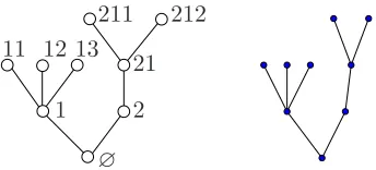
2.3.1 Definition of trees
∅
11 12
211 212
21 13
2 1
Figure 5: A rooted tree and its usual representation on the plane.
Consider the set W = Sn≥0Nn of finite words on the alphabet N = {1,2,3, . . .} where by conventionN0 ={∅}. Foru=u1. . . un, v=v1. . . vm∈W, we let uv=u1. . . unv1. . . vm be the concatenation of the wordsu and v.
Form1, . . . , mp ∈N, we let{m1, . . . , mp}⋆=∪n≥0{m1, . . . , mp}nbe the set of finite words with lettersm1, . . . , mp.
Definition 3. A planar treet is a subset ofW
• containing the root-vertex∅,
• such that ifui∈t for someu∈W and i∈N, then u∈t,
• and such that if ui∈t for some u∈W and i∈N, then uj ∈t for allj∈ {1, . . . , i}.
We denote by T the set of planar trees. For any u ∈ t, let cu(t) = max{i | ui ∈ t} be the number ofchildrenofu. The elements of a treetare callednodes, a node having no child aleaf, the other nodes the internal nodes. The set of leaves of t will be denoted by∂t, and its set of internal nodes byt◦. The number of nodes of a treet is denoted by |t|.
A binary (resp. ternary) treet is a planar tree such thatcu(t)∈ {0,2} (resp. cu(t)∈ {0,3}) for any u∈t. We denote byTbin
and Tter
the set of finite or infinite binary and ternary trees, and by Tbin
n and T ter
n the corresponding set of trees with nnodes.
We now give a formalism to describe the growth of trees. We denote by Tter•
3n+1 := {(t, u) | t∈
Tter
3n+1, u∈∂t}the set of ternary trees with 3n+ 1 nodes with a distinguished leaf. Very similarly with the function Φ defined in Section 2.2, we define the applicationφfromTter•
3k+1 intoT
ter
3k+4 as follows; for any (t, u)∈ Tter•
3k+1, lett′ :=φ(t, u) be the treet∪ {u1, u2, u3}obtained fromtby the replacement of the leafu by an internal node having 3 children.
Definition 4. As for maps (see Definition 1), for any tree t∈ Tter
3k−2, a history of a tree t is a
sequenceh′ =¡(ti, ui), i= 1, . . . , k−1¢ such that(ti, ui)∈ Tter•
3i−2 and ti+1 =φ(ti, ui). The set of
histories of t is denoted byH(t), and we denote HT(k) ={H(t) | t∈ T3terk−2}.
2.3.2 The fundamental bijection between stack-triangulations and ternary trees
Before explaining the bijection we use between△2K andT3terK−2 we define a function Λ which will play an eminent role in our asymptotic results concerning the metrics in maps. LetW1,2,3 be the set of words containing at least one occurrence of each element of Σ3={1,2,3}as for example 321, 123, 113211213123. Letu=u1. . . uk be a word on the alphabet Σ3. Define τ1(u) := 0 and τ2(u) := inf{i|i >0, ui = 1}, the rank of the first apparition of 1 in u. For j≥3, define
τj(u) := inf{i|i > τj−1(u) such thatu1+τj−1(u). . . ui∈W1,2,3}.
This amounts to decomposinguinto subwords, the first one ending when the first 1 appears, the subsequent ones ending each time that each of the three letters 1, 2 and 3 has appeared again. For example ifu= 22123122131 thenτ1(u) = 0, τ2(u) = 3, τ3(u) = 6, τ4(u) = 10. Denote by
Λ(u) = max{i|τi(u)≤ |u|} (1) the number of these non-overlapping subwords. Further for two words (or nodes)u=wa1. . . ak and v=wb1. . . bl witha16=b1, (in this case w=u∧v,) set
Λ(u, v) = Λ(a1. . . ak) + Λ(b1. . . bl). (2)
We call the one or two parameters function Λ the passage function.
We now describe a bijection Ψ△K between△2K and T3terK−2 having a lot of important properties. This bijection is inspired from Darrasse & Soria [16].
Proposition 1. For anyK ≥1 there exists a bijection
Ψ△K : △2K −→ T3terK−2 m 7−→ t:= Ψ△K(m)
such that:
(a) Each internal node u of m corresponds bijectively to an internal nodev of t. We denote for sake of simplicity by u′ the image of u.
(b) Each leaf of t corresponds bijectively to a finite triangular face ofm.
(c) For anyu internal node of m, Λ(u′) =d
m(E0, u). (d) For any u and v internal nodes of m
¯
(e) Let u be an internal node of m. We have
degm(u) = 3 + #{v′∈t◦ |v′=u′w′, w′ ∈1{2,3}⋆∪3{1,2}⋆∪2{1,3}⋆}, (4)
where the set in (4) is the union of the subtrees of t◦ rooted in u′1, u′2 and u′3 formed by the “binary trees” having no nodes containing a 1, resp. a 2, resp a 3.
We will write Ψ△ instead of Ψ△K when no confusion on K is possible.
Property (e) in Proposition 1 is given in Darrasse & Soria [16], where it is used to derive the asymptotic degree distribution of a random node under a Boltzmann distribution (see Section 6). We give below a complete proof of Proposition 1. The quotes around binary trees signal that by construction these branching structures do not satisfy the requirements of Definition 3.
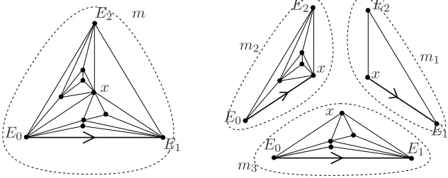
The existence of a bijection between△2K and T3terK−2 is well known and is a simple consequence of the ternary decomposition of the maps in △2K, as illustrated on Figure 6: in the first step of the construction of m, the insertion of the three first edges incident to the node x in the triangle Θ splits it into three parts that behave clearly as stack-triangulations. The nodexmay be recovered at any time since it is the unique vertex incident to the three vertices incident to the infinite face. The bijection induced by this decomposition (this is illustrated on Figure 6)
E0
E0 E0
E1 E1 E1
E2 E2 E2
x x x
x m
m2
m1
m3
Figure 6: Decomposition of a stack-triangulation using the recovering of the first inserted node.
can be defined in order to encode the distance between the nodes in the maps, and then to get the properties announced in Proposition 1. This construction, presented below, is inspired by Darrasse & Soria [16].
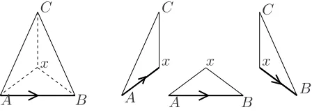
The proof of Proposition 1 we propose raises on an iterative argument, and then will raise on the notion of histories. Since a stack-triangulation generally owns several histories, we need to show some consistence properties of the construction, more or less intuitively clear. The consistence needed relies on an association between the triangular faces of the canonical drawing introduced in Definition 2 and the words on Σ3: thanks to the canonical drawing, there is a sense to talk of a facef without referring to a map, and thanks to our construction of trees, there is a sense to talk of a node u – which is a word – without referring to a tree. We will callcanonical face
Let us now design a bijection ψ△ which associates a word in Σ3 with each canonical face. The image byψ△ of the unique canonical face (E0, E1, E2) of the unique rooted triangle Θ on△2 is
∅, the empty word on Σ3. We now proceed by induction and considerFK the set of canonical faces belonging to at least one of the canonical drawings of a map of△2K. Assume by induction that for any face f inFK, ψ△(f) is well defined and is a word of Σ3. Assume also that there is only one canonical face associated with a geometrical face: if (x1, x2, x3) and (y1, y2, y3) are elements ofFK associated with the same geometrical face, then (x1, x2, x3) = (y1, y2, y3). Let f = (A, B, C) be a canonical face belonging to FK. The growing of a map having f as a face, in the face f, is as explained above, obtained by inserting a node x inf and three edges betweenx and the nodes A, B and C. The three ”new” canonical faces are set to be (B, C, x), (A, x, C), (A, B, x) (this fixes the respected oriented edges, that are chosen in such a way that the infinite face lies on the right of each of these new faces seen as maps, and then allow a successive decomposition, see Figure 7). If the image of f by ψ△ is u, we associate respectively with the three ”new” faces the nodes u1 , u2 and u3. The quotes around ”new” signal that a face in FK may belong also in some Fj for j < K, and then these new faces may ”already” belong toFK. Since the procedure of construction of the faces does not depend on the timeK, the association of u1, u2 and u3 with the new faces is consistent in time. One now can check easily thatψ△ is now defined for any face ofFK+1, and that the properties assumed onFK are inherited inFK+1.
A A
A B B B
C
C C
x x
x x
Figure 7: Heritage of the canonical orientation of the faces. If the first face is sent onu, then the other ones, from left to right are sent onu2, u3 andu1
Now, the bijectionψ△ induces a bijectionψ△K between the setH△(K) of histories of the maps of
△2K andHT(K) the set of histories of the trees of T3terK−2 (for any K≥1). More precisely, the applicationψ△K is defined as follows. The history of the unique stack-triangulation with 4 faces is (Θ,(E0, E1, E2)), and we fix its image to be ({∅},∅) the tree reduced to the root vertex, marked on this node (which is a leaf). Let nowK ≥3 be fixed and lethK =
¡
(mi, fi), i= 1, . . . , K−1¢ be a history of a triangulation mK of △2K. Recall the content of Section 2.2. In particular we have mK = Φ(mK−1, fK−1).
By induction assume that a tree-history h′
K−1 := ¡
(ti, ui), i = 1, . . . , K −2¢ is associated with hK−1:=¡(mi, fi), i= 1, . . . , K−2¢by ψK△−1. Particularly, we assume by induction that for any i≤K−2, ui is given by ψ△(fi) (that is the node marked inti corresponds to the face marked inmi). More globally, thinking to the construction induced by the history, this implies
t◦K−1 ={ψ△(fi) |1≤i≤K−2}. To defineh′
K, we let ½
uK−1 =ψ△(fK−1)
SinceuK−1 =ψ△(fK−1) is a leaf oftK−2,tK−1 is indeed a tree, and alsouK−1 is a leaf oftK−1;
henceh′K :=¡(ti, ui), i= 1, . . . , K−1¢ is a history of a tree, say tK. We then set:
ψ△K(hK) =h′K. (5)
This ends the induction. It turns out thatψK△is a bijection, as stated in the next Lemma. Before stating it, we introduce a notation: ifhK =¡(mi, fi), i= 1, . . . , K−1¢ is a history of mK then for any j < K, we let hj be ¡(mi, fi), i = 1, . . . , j −1¢ the history restricted to the j−1 first steps: hj is the history of a map denoted bymj; accordingly, we do the same for tree-histories.
Lemma 2. For any K≥1,ψK△ is a bijection between H△(K) and HT(K) such that:
(i) The family (ψK△, K ≥1)is consistent: if ψK△(hK) =h′K then for anyj < K,
ψ△j (hj) =h′j.
(ii) Robustness: h(1) and h(2) are two histories of m iff ψK△(h(1)) =ψK△(h(2)) are histories of the same treet.
This Lemma follows easily the construction ofψ△. Now, the point (ii) of this Lemma allows to build an application Ψ△K,⋆ :△2K → T3terK−2 by associating mK withtK (this bijection Ψ△K,⋆ has all the nice properties announced in Proposition 1).
Note 1. We may rephrase what we have done: take any history of a given mapm, and construct iteratively the corresponding ternary tree using ψ△. The last tree obtained does not depend on the history chosen, but only onm.
Lemma 3. Let Ψ△K:△2K → T3terK−2 the application defined above. i) Ψ△K,⋆ is a bijection;
ii) Let t = Ψ△K,⋆(m). The properties assertion (a), (b), (c), (d), (e) of Proposition (1) holds true.
Proof. The application Ψ△K,⋆ is a bijection thanks to the previous Lemma (ii). To prove (ii) of the present Lemma we introduce the notion of type of a face, and of a node (of a word on Σ3). For any face (u, v, w) in m, define
type(u, v, w) := (dm(E0, u), dm(E0, v), dm(E0, w)), (6)
the distance ofu, v, w to the root-vertex ofm. Sinceu,v, and ware neighbors, the type of any triangle is (i, i, i), (i, i, i+ 1), (i, i+ 1, i+ 1) for some i, or a permutation of this.
We then prolong the construction of Φ given above, and mark the nodes of t with the types of the corresponding faces. For any internal nodeu′∈twith type(u′) = (i, j, k),
type(u′1) = ( 1 +i∧j∧k, j, k ), type(u′2) = ( i, 1 +i∧j∧k, k ), type(u′3) = ( i, j, 1 +i∧j∧k )
(7)
E0 E1 E2
Figure 8: Construction of the ternary tree associated with an history of a stack-triangulation
(A, B, C) is translated by the insertion in the tree of the nodes u1 (resp. u2, u3) associated with (x, B, C) (resp. (A, x, B), (A, B, x)). Formula (7) gives then the types of these three faces. Using that type(∅) = (0,1,1),giving t the types of all nodes are known and are obtained via the deterministic evolution rules (7). The distance of any internal node u to the root of m is computed as follows: assume thatu has been inserted at a certain date in a facef = (A, B, C). Then clearly its distance to the root vertex is
dm(E0, u) =g(type(f)),
where g(i, j, k) = 1 + (i∧j ∧k). Moreover, since an internal node in m corresponds to the insertion of three children in the tree, each internal nodeuofmcorresponds to an internal node u′ of tand
dm(E0, u) =g(type(u′)).
It remains to check that for anyu′ ∈t,
g(type(u′)) = Λ(u′) (8)
as defined above. This is a simple exercise: the initial type (that of ∅) varies along a branch of t only when a 1 occurs in the nodes. Then the type passes from (i, i, i) to (i+ 1, i+ 1, i+ 1) when the three letters 1, 2 and 3 has appeared: this corresponds to the incrementation of the distance to the root in the triangulation. This leads to (c).
Note 2. The notion of type of a face f is canonical as we saw, when we proved that it is a function of the ancestors ofu=ψ△(f). Showing this property directly seems a bit ugly.
(d) Consider u and v two internal nodes of m. The node w′ = u′ ∧v′ corresponds to the
smallest canonical facef = (A, B, C) containingu andv. Assumeu′ =w′1. . .and v′ =w′2. . ., then u and v belong respectively to the canonical faces (w, B, C) and (A, w, C). Therefore there exists x ∈ {w, A, B, C} such that dm(u, v) = dm(u, x) +dm(v, x) which leads directly to |dm(u, v)−(dm(u, w) +dm(v, w))| ≤ 2. The remaining cases are treated similarly. Let us investigate now the relation between wand u and Λ(a1. . . aj) in the case where u=wa1. . . aj. Each triangle appearing in the construction ofm behaves as a copy ofm except that its type is not necessarily (i, i+1, i+1) (as was the type of∅). Then the distance of the nodeu=wa1. . . aj towmay be not exactly Λ(a1. . . aj). We now show that
This difference comes from the initialization of the counting of the non-overlapping subwords fromW1,2,3 ina1. . . aj. This counting has to begin when a face of type (i, i, i) has been reached. Since we no longer consider the distance between u and the root but between u and w, the definition of the type has to be slightly modified. Let u = (A, B, C) be the canonical face associated to w′a1. . . aj, we define typew(u) as (dm(A, w), dm(B, w), dm(C, w)).
Let a = a1. . . ak be a word on Σ3. Define τ1′(a) := 1, τ2′(a) := inf{i|i > 1, ai = a1, the rank of the second apparition of a1 ina and τj′(a) =τj(a) for j ≥3 (the definition of τj is given in Equation (39)). Lastly we set
Λw(a) = max{i|τi(a)≤ |a|}.
Let u = wa1. . . aj, it is clear that dm(u, w) = Λw(a1. . . aj) (see the proof of Property (c) of Proposition 1). Furthermore for any wordaon the alphabet Σ3,
|Λ(z)−Λw(z)| ≤1,
which concludes the proof.
(e) Let u be an internal vertex of m and letf = (A, B, C) be the canonical face containingu. Let v be a vertex of m. Then dm(u, v) = 1 if v = A, B, C or if v′ = u′a1. . . aj for a certain a1. . . aj ∈ W3. Assumea1= 1. Then (ψ△)−1(u′a1) = (u, B, C). Nowdm(u, v) = 1 if and only if uis an adjacent vertex to (ψ△)−1(u′a1. . . aj). Furthermore, such a face is of the form (u, B, y), (u, x, y) or (u, x, C) meaning thata2. . . aj ∈ {2,3}⋆ (which can be done by induction). The two remaining casesa1 = 2 anda1 = 3 are done in the same way. ✷
2.4 Induced distribution on the set of ternary trees
The bijection Ψ△K transports the distributionsU△
2K and Q
△
2K on the set of ternary treesT ter
3K−2. 1) First, the distribution
Uter
3K−2:=U△2K◦(Ψ
△
K)−1 (9)
is simply the uniform distribution onTter
3K−2 since Ψ△K is a bijection. 2) The distribution
Qter
3K−2:=Q△2K◦(Ψ
△
K)−1 (10)
is the distribution giving a weight to a tree proportional to its number of histories, that is the number of histories of the corresponding triangulation.
We want to give here another representation of the distributionQter
3K−2.
Definition 5. We call increasing ternary treet= (T, l) a pair such that:
• T is the set of internal nodes of a ternary tree,
• l is a bijective application between T (viewed as a set of nodes) onto {1, . . . ,|T|} such that l
is increasing along the branches (thus l(∅) = 1).
Notice thatT is not necessarily a tree as defined in Section 2.3.1: for example T may be{∅,2}. LetIter
K denotes the set of increasing ternary trees (T, l) such that|T|=K (i.e. T is the set of internal nodes of a tree inTter
The number of histories of a ternary treet∈ Tter
3K−2 is given by the
wK−1(t◦) = #{(t◦, l)∈ IKter−1}
the number of increasing trees havingt◦as first coordinate, in other words, with shapet◦. Indeed in order to record the number of histories oftan idea is to mark the internal nodes oftby their apparition time, the root being marked 1. Hence the marks are increasing along the branches, and there is a bijection between{1, . . . , K−1}and the set of internal nodes oft. Conversely, any labeling oft◦ with marks having these properties corresponds indeed to a history ofm. Thus
Lemma 4. For any K≥1, the distributionQter
3K−2 has the following representation
Qter
3K−2(t) =CK−1·wK−1(t◦), for anyt∈ T
ter
3K−2
where CK−1 is the constant CK−1 :=³Pt′∈Tter
3K−2wK−1(t
′◦)´−1.
3
Topologies
3.1 Topology of local convergence
The topology induced by the distancedL defined below will be called “topology of local conver-gence”. Its aim is to describe an asymptotic behavior of maps (or more generally graphs) around their root. We stress on the fact that no rescaling is involved in this part.
We borrow some considerations from Angel & Schramm [5]. Let Mbe the set of rooted maps (m, e) wheree= (E0, E1) is the distinguished edge ofm. The maps fromMare not assumed to be finite, but only locally finite, i.e. the degree of the vertices are finite. For anyr ≥0, denote by Bm(r) the map having as set of vertices
V(Bm(r)) ={u∈V(m) |dm(u, E0)≤r},
the vertices inm with graph distance toE0 non greater thanr, and having as set of edges, the edges in E(m) between the vertices of V(Bm(r)).
For anym= (m1, e) andm′= (m′, e′) in Mset
dL(m, m′) = 1/(1 +k) (11)
wherekis the supremum of the radiusrsuch thatBm(r) andBm′(r) are equals as rooted maps. The application dL is a metric on the space M. A sequence of rooted maps converges to a given rooted map m (for the metricdL) if eventually they are equivalent with m on arbitrarily large combinatorial balls around their root. In this topology, all finite maps are isolated points, and infinite maps are their accumulation points. The space Mis complete for the distance dL since given a Cauchy sequence of locally finite embedded rooted maps it is easy to see that it is possible to choose for them embeddings that eventually agree on balls of any fixed radius around the root. Thus, the limit of the sequence exists (as a locally finite embedded maps). In other words, the spaceT of (locally finite embedded rooted) maps is complete.
3.2 Gromov-Hausdorff topology
The other topology we are interested in will be the suitable tool to describe the convergence of rescaled maps to a limiting object. The point of view here is to consider maps endowed with the graph distance as metric spaces. The topology considered – called the Gromov-Hausdorff topology – is the topology of the convergence of compact (rooted) metric spaces. We borrow some considerations from Le Gall & Paulin [32] and from Le Gall [30, Section 2]. We send the interested reader to these works and references therein.
First, recall that the Hausdorff distance in a metric space (E, dE) is a distance between the compact sets of E; forK1 and K2 compacts inE,
dHaus(E)(K1, K2) = inf{r |K1 ⊂K2r, K2 ⊂K1r}
where Kr =∪
x∈KBE(x, r) is the union of open balls of radiusr centered on the points of K. Now, given two pointed (i.e. with a distinguished node) compact metric spaces ((E1, v1), d1) and ((E2, v2), d2), the Gromov-Hausdorff distance between them is
dGH(E1, E2) = inf{dHaus(E)(φ1(E1), φ2(E2))∨dE(φ1(v1), φ2(v2))},
where the infimum is taken on all metric spacesE and all isometric embeddingsφ1 andφ2 from (E1, d1) and (E2, d2) in (E, dE). Let K be the set of all isometric classes of compact metric spaces, endowed with the Gromov-Hausdorff distance dGH. It turns out that (K, dGH) is a complete metric space, which makes it appropriate to study the convergence in distribution of
K-valued random variables.
The Gromov-Hausdorff convergence is then a consequence of any convergence ofEn′ toE∞′ , when E′
n andE∞′ are some isomorphic embeddings ofEnand E∞in a common metric space (E, dE). In the proofs, we exhibit a space (E, dE) where this convergence holds; hence, the results of convergence we get are stronger than the only convergence for the Gromov-Hausdorff topology. In fact, it holds for a sequence of parametrized spaces.
4
Local convergence of stack-triangulations under
U
△2nWe first begin by giving some information about Galton-Watson trees conditioned by the size. These facts will be used also in Section 5.
4.1 Galton-Watson trees conditioned by the size
Considerνter:= 23δ0+13δ3as a (critical) offspring distribution of a Galton-Watson (GW) process
starting from one individual. Denote byPter
the law of the corresponding GW family tree; we will also writePter
n instead ofP ter¡
.¯¯|t|=n¢.
Lemma 5. Pter
3n+1 is the uniform distribution on T
ter
3n+1.
Proof. A ternary treet with 3n+ 1 nodes hasn internal nodes having 3 children and 2n+ 1 leaves with degree 0. Hence Pter
3n+1({t}) = 3−n(2/3)2n+1/P
ter
(Tter
3n+1). This is constant onT
ter
3n+1 and has supportTter
The conclusion is that for anyK ≥1
Pter
3K−2 =U
ter
3K−2. (12)
Following (9), this gives us a representation of the uniform distribution on Tter
3K−2 in terms of conditioned GW trees. This will be our point of view in the sequel of the paper.
We would like to point out that the number of ternary trees with a given number of nodes, as well as the number of forests #Fterr (k) of ternary trees withr roots and a total number of nodes K are well known:
These formulas are consequence of the so-called rotation/conjugation principle due to Raney, or Dvoretzky-Motzkin (see Pitman [42], Section 5.1 for more information on this principle).
We now state some results concerning the local convergence of uniform ternary trees. The limiting random tree will be used to build the limiting random maps, local limit of stacked-triangulations.
4.2 Local convergence of uniform ternary trees
We endowTter
with the local distancedLdefined in (11): instead of redefining an ad hoc metric similar todL on the set of planar trees, we identify the set of trees with the set of rooted planar maps with one face (this is classical, and corresponds to the embedding of planar trees in the plane respecting the cyclical order around the vertices). Under this metric, the accumulation points of sequences of trees (tK) such that |tK| = 3K−2 are infinite trees. It is known that the sequence (Pter
3K−2) converges weakly for the topology of local convergence. Let us describe a random tree tter∞ under the limit distribution, denoted byPter
∞.
LetW3 be the infinite complete ternary tree and let (Xi) be a sequence of i.i.d. r.v. uniformly distributed on Σ3. Define
obtained istter∞. In the literature the branchLter
∞ is called thespineor theinfinite line of descent
intter
∞.
Proposition 6. (Gillet [23]) When n →+∞, Pter
3n+1 converges weakly to P
ter
∞ for the topology
of local convergence.
This result is due to Gillet [23, Section III] (see Theorems III.3.1, III.4.2, III.4.3, III.4.4).
Note 3. The distributionPter
∞ is usually called “size biased GW trees”. We send the interested
4.3 Local convergence of stacked-triangulations
The first aim of this part is to define a mapm∞ built thanks totter∞ with the help of a limiting
“bijection” analogous to the functions Ψ△K’s. Some problems arise when one wants to draw or define an infinite map on the plane since we have to deal with accumulation points and possible infinite degree of vertices. We come back on this point in Section 4.3.1. We now describe a special class of infinite trees – we call themthin ternary trees– that will play an important role further.
Definition 6. An infinite line of descent in a tree is a sequence(ui, i≥0) such that: u0 is the
root ∅, and ui is a child of ui−1 for any i≥1. We call thin ternary tree a ternary tree having a
unique infinite line of descent L= (ui, i≥0), satisfying moreover Λ(un)−→
n ∞ (which will be
written Λ(L) =∞). The set of thin ternary trees is denoted by Tter thin.
Lemma 7. The support ofPter
∞ is included in T
ter thin.
Proof. By constructionLter
∞ is an infinite line of descent int
ter
∞ that satisfies clearly a.s. Λ(L
ter
∞) =
+∞. This line is a.s. unique because the sequence (t(i)) of grafted trees are critical GW trees
and then have a.s. all a finite size. ✷
For any treet, finite or not, denote the Λ−ball oft of radius r by
BrΛ(t) :={u |u∈t,Λ(u)≤r}.
Lemma 8. For any treet∈ Tter
thin and any r ≥0, #BrΛ(t) is finite.
Proof. LetLbe the unique infinite line of descent oft. Since Λ(L) = +∞,BrΛ(t) contains only a finite part sayJ∅, uKofL. This part is connected since Λ is non decreasing: ifw=uv for two wordsu and v then Λ(w) ≥Λ(u). Using again that Λ is non decreasing,BΛ
r(t) is contained in
J∅, uKunion the finite set of finite trees rooted on the neighbors ofJ∅, uK. ✷
Proposition 9. If a sequence of trees(tn) converges for the local topology to a thin tree t, then
for anyr ≥0 there existsNr such that for any n≥Nr, BrΛ(tn) =BrΛ(t).
Proof. Suppose that this is not true. Then take the smallest r for which there does not exists such a Nr (then r ≥1 since the property is clearly true for r = 0). Let lr be the length of the longest word in BΛ
r(t). Since dL(tn, t) ≤ 1/(lr+ 1) for n say larger than Nr′, for those n the words in tn and t with at most lr letters coincide. This implies that BrΛ(t)⊂BΛr(tn) and that this inclusion is strict for a sub-sequence (tnk) of (tn). Hence one may find a sequence of words
wnk such that: Λ(wnk) =r,wnk ∈tnk,wnk ∈/ t. Let wn′k be the smallest (for the LO) elements
of (tnk) with this property. In particular, the fatherw
f
nk ofw′nk satisfies either:
(a) Λ(wnfk) =r−1 or,
(b) Λ(wfnk) =r and thenw
f
nk belongs toB
Λ r(t).
For n large enough, say larger thanNr−1, BΛr−1(tn) coincides with BΛr−1(t) (since r is the first number for which this property does not hold). Hence, the setSf ={wfnk |nk≥Nr−1∧N
′
r} ⊂ BΛ
r(t) is finite by the previous Lemma. Then the sequence (w′nk) takes its values in the set of
children of the nodes of Sf, the finite set say Sr. Consider an accumulation point p of (w′nk).
4.3.1 A notion of infinite map
This section is much inspired by Angel & Schramm [5] and Chassaing & Durhuus [13, Section 6].
We call infinite map m, the embedding of a graph in the plane having the following properties:
(α) it is locally-finite, that is the degree of all nodes is finite,
(β) if (ρn, n≥1) is a sequence of points belonging to distinct edges of m, then accumulation points of (ρn) are not on m(neither on the edges or on the vertices ofm).
This last condition ensures that no face is created artificially. For example, we want to avoid a drawing of an infinite graph where each node has degree 2 (an infinite graph line, in some sense) that would create two faces or more, as would result by a drawing of this graph where the two extremities accumulate on the same point. Avoiding the creation of artificial faces allows to ensure that homeomorphisms of the plane are still the right tools to discriminate similar objects. In the following we define an application Ψ△∞ that associates with a tree t of Tthinter an infinite
map Ψ∞△(t) of the plane. Before this, let us make some remarks. Lett∈ Tthinter, for anyr, sett(r)
the tree having as set of internal nodesBrΛ=BΛr(t). We have clearlydL(t(r), t)→
r 0. Moreover, sincet(r) is included int(r+ 1), the mapmr= (Ψ△)−1(t(r)) is “included” inmr+1. The quotes are there to recall that we are working on equivalence classes modulo homeomorphisms and that the inclusion is not really defined stricto sensu. In order to have indeed an inclusion, an idea is to use the canonical drawing (see Definition 2) : the inclusionG(mr)⊂ G(mr+1) is clear if one uses a history leading to mr+1 that passes frommr, which is possible thanks to Property (i) of Proposition 2 and the fact thatt(r)⊂t(r+ 1). Now (G(mr)) is a sequence of increasing graphs. LetGtbe defined as the map ∪rG(mr) and having as set of nodes and edges those belonging to at least one of theG(mr).
Proposition 10. For any thin tree t, the map Gt satisfies(α) and (β).
Proof. The first assertion comes from the construction and the finiteness of the balls BΛ r (by Lemma 8). For the second assertion, just notice that for any r, only a unique face of mr contains an infinite number of faces of Gt. Indeed, t(r) is included in t and t owns only one infinite line of descent L. Hence among the set of fringe subtrees {tu | u ∈ t(r)} of t (each of them corresponding to the nodes that will be inserted in one of the triangular faces ofmr) only one has an infinite cardinality. It remains to check that the edges do not accumulate, and for this, we have only to follow the sequence of triangles (Fk) that contains an infinite number of faces, those corresponding with the nodes of L. Moreover, by uniqueness of the infinite line of descent int, the family of triangles (Fk) forms a decreasing sequence for the inclusion. Consider now the subsequenceFnk whereg(type(Fnk)) = g(type(Fnk−1)) + 1. The triangle Fnk has then
all its sides different from Fnk−1. Hence any accumulation points ρ of (ρn) (as defined in (β))
must belong to∩Fk. By the previous argument, ρdoes not belong to any side of those triangles, which amounts to saying thatρ lies outside m. ✷
Proposition 11. Let (tn) be a sequence of trees, tn ∈ Tter
3n−2, converging for the local topology
Proof. If (tn) converges totthen for anyr, there existsnr such that for anyn≥nr,BrΛ(tn) = BΛ
r(t). Hence, ifnis large enough, dL((Ψ△n)−1(tn),Gt)≤1/(r+ 1). ✷ We have till now, work on topological facts, separated in some sense from the probabilistic considerations. It remains to deduce the probabilistic properties of interest.
4.3.2 A law on the set of infinite stack-maps
The set Tter
is a Polish space for the topology dL. In such a space, Skorohod’s representation theorem (see e.g. [27, Theorem 4.30]) applies. SincePter
3n−2 converges toP
ter
∞, there exists a space
Ω on which are defined altogether ˜t∞,˜t1,˜t2, . . ., such that ˜tn ∼ P3tern−2 for any n, ˜t∞ ∼ P∞ter,
and such that ˜tn (a.s.)
−−−→n ˜t∞. Moreover, thanks to Lemma 7, ˜t∞ is a.s. a thin tree.
We then work on this space Ω and use the almost sure properties of ˜t∞. The convergence in
distribution of our theorem will be a consequence of the a.s. convergence on Ω.
Definition 7. We denote by P∞△ the distribution ofm∞:=Gt∞.
A simple consequence of Proposition 11 is the following assertion. SincedL(˜tn,˜t∞)
(a.s.)
−−−→n 0 then
dL ³
(Ψ△n)−1(˜tn),G˜t∞ ´ (a.s.)
−−−→n 0. (15)
This obviously implies the following result.
Theorem 12. (U△
2n) converges weakly to P∞△ for the topology of local convergence.
5
Asymptotic under the Gromov-Hausdorff topology
The asymptotic behavior of GW trees underPter
n is very well studied. We focus in this section on the limiting behavior under the Gromov-Hausdorff topology. The facts described here will be used later in the proof of the theorems stating the convergence of stack-triangulations. In addition we stress on the fact that the limit of rescaled stack-maps under the uniform distribution is the same limit as the one of GW trees: the continuum random tree.
5.1 Gromov-Hausdorff convergence of rescaled GW trees
We present here the limit of rescaled GW trees conditioned by the size for the Gromov-Hausdorff topology. We borrow some considerations from Le Gall & Weill [33] and Le Gall [30].
We adopt the same normalizations as Aldous [1; 2]: the Continuum Random Tree (CRT)T2ecan
be defined as the real tree coded by twice a normalized Brownian excursione= (et)t∈[0,1]. Indeed, any functionf with duration 1 and satisfying moreoverf(0) =f(1) = 0, andf(x)≥0, x∈[0,1] may be viewed as coding a continuous tree as follows (illustration can be found on Figure 9). For everys, s′ ∈[0,1], we set
mf(s, s′) := inf
We then define an equivalence relation on [0,1] by setting s ∼ f s
′ if and only if f(s) = f(s′) =
mf(s, s′). Finally we put
df(s, s′) =f(s) +f(s′)−2mf(s, s′) (16) and note thatdf(s, s′) only depends on the equivalence classes of sand s′.
0 s s′ t 1
f(s) f(t)
mf(s, t)
Figure 9: Graph of a continuous functionf satisfyingf(0) =f(1) = 0andf(x)≥0 on [0,1]. In this example s ∼
f s
′ and the distancedf(s, t) =df(s′, t) =f(s) +f(t)−2mf(s, t) is the
sum of the lengths of the vertical segments.
Then the quotient space Tf := [0,1]/ ∼
f equipped with the metric df is a compact R-tree (see e.g. Section 2 of [18]). In other words, it is a compact metric space such that for any two points σ andσ′ there is a unique arc with endpointsσ andσ′ and furthermore this arc is isometric to a
compact interval of the real line. We viewTf as a rooted R-tree, whose root ρis the equivalence class of 0.
The CRT is the metric space (T2e, d2e). In addition to the usual genealogical order of the tree,
the CRTT2einherits a LO from the coding by 2e, in a way analogous to the ordering of (discrete)
plane trees from the left to the right.
Discrete trees T are now equipped with their graph distancesdT.
Proposition 13. The following convergence holds for the GH topology. UnderPter
3n+1, Ã
T,pdT 3n/2
! (d)
−−→
n (T2e, d2e).
Proof. The convergence for the GH topology is a consequence of the convergence for any suitable encoding of trees. The offspring distributionνter:= 23δ0+13δ3 is critical (in other words
has mean 1) and variance 2. The convergence of rescaled GW trees conditioned by their size is proved by Aldous [1; 2]. (See also Le Gall [30] or Marckert & Mokkadem [38], Section 6 of
Pitman [42]). ✷
5.2 Gromov-Hausdorff convergence of stack-triangulations
Lemma 14. Let (Xi)i≥1 be a sequence of random variables uniform in Σ3 = {1,2,3}, and
independent. LetWn be the word X1. . . Xn. (i) n−1Λ(Wn)
(a.s.)
−−−→n Λ△ where
Λ△:= 2/11. (17)
(ii) P(|Λ(Wn)−nΛ△| ≥n1/2+u)→
n 0 for anyu >0.
Proof. If W is the infinite sequence (Xi), clearly τ2(W) ∼Geometric(1/3) and for i ≥3, the (τi(W)−τi−1(W))′sare i.i.d., independent also fromτ2, and are distributed as 1+G1+G2where G1 ∼ Geometric(1/3) and G2 ∼ Geometric(2/3) [the distribution Geometric(p) is Pk≥1p(1− p)k−1δk]. It follows that E(τi(W)−τi−1(W)) = 11/2 for i≥3 and E(τ2(W)) = 3 <+∞. By the renewal theorem assertion (i) holds true. For the second assertion, write
{|Λ(Wn)−nΛ△| ≥n1/2+u}={τnΛ△+n1/2+u ≤n} ∪ {τnΛ△−n1/2+u ≥n}.
By the Bienaym´e-Tchebichev inequality the probability of the events in the right hand side goes
to 0. ✷
For every integer n≥2, let Mn be a random rooted map under U△2n. Denote bymn the set of vertices ofMn and bydmn the graph distance onmn. We view (mn, dmn) as a random variable
taking its values in the space of isometric classes of compact metric spaces.
Theorem 15. Under U△
2n, Ã
mn, dmn
Λ△
p 3n/2
! (d)
−−→n (T2e, d2e),
for the Gromov-Hausdorff topology on compact metric spaces.
This theorem is a corollary of the following stronger Theorem stating the convergence of maps seen as parametrized metric spaces. In order to state this theorem, we need to parametrize the map Mn. The set of internal nodes of mn inherits of an order, the LO on trees, thanks to the function Ψ△n. Letu(r) be therth internal node ofmnforr ∈ {0, . . . , n−1}. Denote bydmn(k, j)
the distance betweenu(k) andu(j) inmn. We need in the following theorem to interpolatedmn
between the integer points to obtain a continuous function. Any smooth enough interpolation is suitable. [For example, define dmn as the plane interpolation on the triangles with integer
coordinates of the form (a, b),(a+ 1, b),(a, b+ 1) and (a, b+ 1),(a+ 1, b+ 1),(a+ 1, b)].
Theorem 16. Under U△
2n, Ã
dmn(ns, nt)
Λ△
p 3n/2
!
(s,t)∈[0,1]2
(d)
−−→n (d2e(s, t))(s,t)∈[0,1]2, (18)
where the convergence holds in C[0,1]2 (even if not indicated, the space C[0,1] and C[0,1]2 are
The proof of this Theorem is postponed to Section 9.1.
Proof of Theorem 15. To explain why Theorem 15 is a consequence of Theorem 16, we introduce the notion of correspondence between two pointed compact metric spaces. Let ((E, v), d) and ((E′, v′), d′) be two pointed compact metric spaces. We say that R ⊂E×E′ is a correspondence between ((E, v), d) and ((E′, v′)d′) if (v, v′) ∈ R and for every x ∈ E (resp.
x′ ∈ E′) there exists y′ ∈ E′ (resp. y ∈ E) such that (x, y′) ∈ R (resp. (x′, y) ∈ R). The distorsion ofRis defined by
dis(R) = sup©|d(x, y)−d′(x′, y′)| : (x, x′),(y, y′)∈ Rª.
It has been proved in [19] that
dGH(E, E′) = 1
2inf{dis(R) : R ∈ C}, (19) whereC denotes the set of all correspondences between ((E, v), d) and ((E′, v′), d′).
Letmnbe a uniform stack-triangulation with 2nfaces. Then one can construct a correspondence
Rnbetween ((mn, E0), dmn/Λ△
p
3n/2) and a continuous treeT2ethanks to the parametrization
ofmn, that is
Rn={(u(ns), s)∈mn× T2e : s∈[0,1]}.
Now using Theorem 16, by Skorohod’s representation theorem there exists a space Ω where a copy dgmn of dmn, and a copy ˜d2e of d2e satisfies dm˜n
(a.s.)
−−−→n df2e in C[0,1]2. On this space the
correspondence dis(Rfn) = sup{|dmgn(ns, nt)/Λ△
p
3n/2−df2e(s, t)| : (s, t) ∈ [0,1]2}. On the
space Ω, a.s. dis(Rfn)→0, which implies Theorem 15 (together with (19)). ✷
The profile Profm := (Profm(t), t≥0) of a mapm with root vertex E0 is the c`adl`ag-process
Profm(t) = #{u∈V(m) |dm(E0, u)≤t}, for anyt≥0.
The radiusR(m) = max{dm(u, E0) |u∈V(m)} is the largest distance to the root vertex inm. As a corollary of Theorem 15 or Theorem 16, we have:
Corollary 17. Under U△2n, the process
³
n−1Profmn(Λ△
p
3n/2v)´ v≥0
(d)
−−→n
µZ v
0 lx2edx
v≥0
(20)
where lx
2e stands for the local time of twice the Brownian excursion 2e at position x at time 1,
and where the convergence holds in distribution in the setD[0,+∞)of c`adl`ag functions endowed with the Skorohod topology. Moreover
R(mn) Λ△
p 3n/2
(d)
−−→n 2 maxe
Proof. Let Dn(s) = dmn(ns,0) Λ△√3n/2
be the interpolated distance to E0. By (18), (Dn(s))s∈[0,1] (d)
−−→
copy ˜Dn ofDn, and a copy ˜e ofesatisfies ˜Dn−−−→(a.s.) C[0,1]. This yields the convergence of Profmn as asserted in (20).
For the second assertion, note that f →maxf is continuous onC[0,1]. Since ˜Dn−−−→(a.s.)
n 2˜ethen max ˜Dn
(a.s.)
−−−→n max 2e, and then also in distribution. ✷
6
Asymptotic behavior of the typical degree
The results obtained in this part are summed up in the following Proposition.
Proposition 18. Let mn be a map U△2n distributed, u(1) the first node inserted in mn, and u
be a random node chosen uniformly among the internal nodes of mn. (i) degmn(u(1))−−→(d)
The (ii) point has been shown by Darrasse & Soria [16], in the case of a model of stack-triangulations under a Boltzmann model. Assertion (ii) follows nevertheless their work, and a technical lemma saying that in a Galton-Watson tree t conditioned to have a total size n with offspring distribution νter, the fringe subtree tu taken at a random node u, converges
in distribution to a Galton-Watson tree under νter (with no conditioning) when n → +∞.
This argument should be detailed in a forthcoming work of Darrasse & Soria. We give below an elementary proof of this Lemma avoiding the Boltzmann distribution, and the generating function.
Lemma 19. Let T be a random tree under Uter
3n+1 and u be chosen uniformly in T◦. We have
, for k ≥ 1. Moreover, conditionally on
|Tu|=m,Tu has the uniform distribution inT
Note 4. There are several ways to check that the limiting sequences in Proposition 18 and Lemma 19 define indeed some probability distributions. One may use an approach using gener-ating functions. Alternatively, one may use probabilistic arguments.
For the sum in the Lemma, proceed as follows: Consider the family tree of a Galton-Watson process with the critical offspring distribution νter starting from one individual. Each of the
1 3k+1
¡3k+1 k
¢
ternary trees having3k+1nodes, has weight 2323kk+1+1 under this law. The a.s. extinction
of this Galton-Watson process rewrites Pk≥133k2(32kk+1+1) individuals: since it is sub-critical, this probability is 1.
A probabilistic proof of Pk≥1k+3k ¡2kk+2¢322kk+3+3 = 1 runs as follows: one checks that this sum
equals 13Pk≥0P(S2k+4 =−4) where Sj is a sum of j i.i.d. random variables taking values −1
or +1 with probability 2/3 and 1/3. Then Pk≥0P(S2k+4 = −4) = E(Pj1S
j=−4) is the mean
time passed by the random walkS, at position −4: the identity is exact since −4 can be reached only at even dates. But the mean sojourn time in a given position with negative ordinate is 3, since the drift of the random walk is −1×(2/3) + 1×(1/3) =−1/3.
the set of ternary trees with a distinguished internal node, resp. leaf. For any tree t and u ∈ t set t[u] = {v ∈ t | v is not a descendant of u}. Each element (t, u) of Tter⋆
3n+1 can be decomposed bijectively as a pair [(t[u], u), tu] where (t[u], u) is a tree with a marked leaf, andtu is a ternary tree having at least one internal node. Hence, for any n, the functionρ defined by ρ(t, u) := [(t[u], u), tu] is a bijection fromT3tern+1⋆ onto
3n+1 have the same number of internal nodes, choosing a treeT uniformly in
Tter
To conclude that we have indeed a convergence in distribution of degT(u) under Uter
3n+1 to K, we use that the limit sums to 1 (see Note 4). The second assertion of the Lemma is clear. ✷
Proof of Proposition 18. As illustrated on Figure 10, for anyt∈ Tter
, we let
tdeg :={v|v ∈t, v∈1{2,3}⋆∪2{1,3}⋆∪3{1,2}⋆}.
Figure 10: A ternary tree tandtdeg. Plain vertices belong totdeg.
3. For sake of compactness, we will however up to a slight abuse of language call these three pseudo-trees, binary trees (combinatorially their are binary trees).
(i) LetT be a tree Uter not reduced to the root vertex can be decomposed in a unique way as a pair (tdeg, f) where f := (t(1), . . . , t(k))∈(Tter
)kis a forest of ternary trees, andk= #(tdeg∩t◦). LetFbinn (k) (resp
Ftern (k)) be the set of forests composed withnbinary (resp. ternary) trees and total number of
nodesk. For 0≤k < n−1, we get:
A well known consequence of the rotation/conjugation principle (see Pitman [42] Section 5.1) is that
with the convention that¡ab¢ is 0 ifbis negative or non integer. We then have
Uter
32k+3, limit which is indeed a probability
distri-bution (see Note 4).
Conditioning on |Tu′|, using Formulas (22) and (27) we get after simplification
where
which is the probability distribution announced to be the limit ofqn,k. To end the proof we have to explain why the exchange limn and Pj≥k+2 is legal.
By Fatou’s lemma, for anyk one has
lim sup
7
Asymptotic behavior of stack-triangulations under
Q
△2nWe first present a result concerning ternary trees underQter
3n−2.
Proposition 20. Let t be a random tree under Qter
3n−2, and u and v be two nodes chosen
uni-formly and independently in t◦; let w=u∧v be their deepest common ancestor. 1) We have ¡32logn¢−1/2¡|u| − 32logn,|v| − 32logn¢ −−→(d)
n (N1, N2) where N1 and N2 are
inde-pendent centered Gaussian r.v. with variance 1.
2) Let a0. . .ak andb0. . .bl be the unique words such that u=wa0. . .ak and v=wb0. . .bl.
The following theorem may be considered as the strongest result of this section. As explained in its proof, it is an immediate consequence of Proposition 20.
Theorem 21. Let Mn be a stack-triangulation underQ△2n. Letk∈Nand v1, . . . ,vk be knodes
![Figure 9: Graph of a continuous function f satisfying f(0) = f(1) = 0 and f(x) ≥ 0 on [0,1].In this example s ∼f s′ and the distance df(s, t) = df(s′, t) = f(s) + f(t) − 2 mf(s, t) is the](https://thumb-ap.123doks.com/thumbv2/123dok/984021.916782/22.612.183.415.169.273/figure-graph-continuous-function-satisfying-example-distance-df.webp)