ELECTRONIC
COMMUNICATIONS in PROBABILITY
GRAPHICAL REPRESENTATION OF SOME
DUALI-TY RELATIONS IN STOCHASTIC POPULATION
MO-DELS
ROLAND ALKEMPER
Department of Mathematics, Johannes-Gutenberg Universit¨at, Staudingerweg 9, 55099 Mainz, Germany
email: [email protected]
MARTIN HUTZENTHALER
Department of Mathematics and Computer Science, Universit¨at Frankfurt, Robert-Mayer-Str. 6-10, 60325 Frankfurt am Main, Germany
email: [email protected]
Submitted September 4, 2006, accepted in final form June 5, 2007 AMS 2000 Subject classification: 60K35
Keywords: Duality, graphical representation, Feller’s branching diffusion, branching-coalescing particle process, resampling-selection model, stochastic population dynamics
Abstract
We derive a unified stochastic picture for the duality of a resampling-selection model with a branching-coalescing particle process (cf. [1]) and for the self-duality of Feller’s branching diffusion with logistic growth (cf. [7]). The two dual processes are approximated by particle processes which are forward and backward processes in a graphical representation. We identify duality relations between the basic building blocks of the particle processes which lead to the two dualities mentioned above.
1
Introduction
Two processes (Xt)t≥0 and (Yt)t≥0 with state spacesE1 andE2, respectively, are called dual
with respect to the duality function H if H: E1×E2 → R is a measurable and bounded
function and if Ex[H(X
t, y)] =Ey[H(x, Yt)] holds for all x∈E1, y ∈E2 and allt ≥0 (see
e.g. [9]). Here superscripts as in Px or inEx indicate the initial value of a process. In this paper,E1 andE2will be subsets of [0,∞) or will be equal to{0,1}N. We speak of amoment
duality ifH(x, y) =yxorH(x, y) = (1−y)x,x∈E
1⊂N0,y∈[0,1], and of aLaplace duality
ifH(x, y) = exp (−λx·y),x, y∈E1=E2⊂[0,∞), for someλ >0.
We provide a unified stochastic picture for the following moment duality and the following Laplace duality of prominent processes from the field of stochastic population dynamics. For the moment duality, let b, c, d ≥ 0. Denote by Xt ∈ N0 the number of particles at time
t ≥ 0 of the branching-coalescing particle process defined by the initial value X0 = n and
at rate d and each ordered pair of particles coalesces into one particle at rate c. All these events occur independently of each other. In the notation of Athreya and Swart [1], this is the (1, b, c, d)-braco-process. Its dual process (Yt)t≥0 is the unique strong solution with values in
[0,1] of the one-dimensional stochastic differential equation
dYt= (b−d)Ytdt−bYt2dt+
p
2cYt(1−Yt) dBt, Y0=y, (1)
where (Bt)t≥0 is a standard Brownian motion. Athreya and Swart [1] call this process the
resampling-selection process with selection rate b, resampling rate c and mutation rated, or shortly the (1, b, c, d)-resem-process. They prove the moment duality
En
(1−y)Xt=Ey(1
−Yt)n
∀n∈N0, y∈[0,1], t≥0. (2)
For the Laplace duality, let (Xt)t≥0 denote Feller’s branching diffusion with logistic growth,
i.e., the strong solution of
dXt=αXtdt−γXt2dt+
p
2βXtdBt, (3)
where α, γ, β ≥ 0 and (Bt)t≥0 is a standard Brownian motion. We call this process the
logistic Feller diffusion with parameters (α, γ, β). Let (Yt)t≥0 be a logistic Feller diffusion
with parameters (α, rβ, γ/r) for somer >0. Hutzenthaler and Wakolbinger [7] establish the Laplace duality
Ex
e−rXt·y=Eye−rx·Yt,
∀x, y∈[0,∞), t≥0. (4) The duality relations (2) and (4) include as special cases (see Remark 4.2 and Remark 4.4) the Laplace duality of Feller’s branching diffusion with a deterministic process, the moment duality of the Fisher-Wright diffusion with Kingman’s coalescent, and the moment duality of the (continuous time) Galton-Watson process with a deterministic process.
In the references [1] and [7], the duality relations (2) and (4) are proved analytically by means of a generator calculation. In this paper, we take a different approach by explaining the dynamics of the processes viabasic mechanismson the level of particles which lead to the above dualities. To this end, for every N ∈ N, we construct approximating Markov processes X
N t
t≥0 and YN
t
t≥0with c`adl`ag sample paths and state space{0,1}
N and with the following properties.
The processes (XN
t )t≥0and (YtN)t≥0 are dual in the sense that
PxN
XtN∧yN = 0
=PyN
xN ∧YtN = 0
, ∀xN, yN ∈ {0,1}N ∀t≥0. (5)
The notationxN∧yN denotes component-wise minimum and 0 denotes the zero configuration. If|XN
0 |=n, for some fixedn≤N, then |XtN|
t≥0converges weakly to a branching-coalescing
particle process asN → ∞. We use the notation|xN|:=PN
i=1xNi forxN ∈ {0,1}N. Assume that the set of c`adl`ag-paths is equipped with the Skorohod topology (see e.g. [4]). Ifn=n(N) depends onN such thatn/N→x∈[0,1] asN → ∞, then (|XN
t |/N)t≥0converges weakly to
a resampling-selection model. If n=n(N) satisfies n/√N → x≥0, then |XN t√N|/
√
N
t≥0
converges weakly to Feller’s branching diffusion with logistic growth. The process (YN t )t≥0
differs from (XN
t )t≥0 only by the set of parameters and by the initial condition.
We will derive the moment duality (2) and the Laplace duality (4) from (5) in the following way. Let the random variable XN
0 be uniformly distributed over all configurations xN ∈ {0,1}N
Similarly, choose YN
0 uniformly in{0,1}N with|Y0N|=k=k(N) for a givenk(N)≤N. We
will prove in Proposition 3.1 that property (5) implies a prototype duality relation, namely
lim N→∞E
h
1−Nki
XtTNN
= lim N→∞E
h
1−
YtTNN
N
i
n
, t≥0, (6)
under some assumptions – including the convergence of both sides – on the two processes and on the sequence (TN)N≥1⊂R
≥0. Choosingnfixed,ksuch that Nk →y≥0 and lettingTN = 1, we deduce from (6) (and from the convergence properties of (XtN)t≥0 and of (YtN)t≥0) the
moment duality of a branching-coalescing particle process with a resampling-selection model (cf. Theorem 4.1). In order to obtain a Laplace duality of logistic Feller diffusions, choosen, k
such that √n
N →x≥0, k
√
N → y ≥0 and TN = √
N. Notice that (1−√y
N) x√N
converges to e−xy uniformly in 0≤x, y ≤x˜ as N → ∞ for every ˜x≥0. This together with the weak convergence of the rescaled processes will imply
lim N→∞E
h
e−|X N t√N|·y
√
Ni
= lim N→∞E
h
e−x·|Y N t√N|
√
Ni
. (7)
For the construction of the approximating processes, we interpret the elements of {1, . . . , N} as “individuals” and the elements of {0,1}as the “type” of an individual. In the terminology of population genetics, individuals are denoted as “genes”, whereas in population dynamics, the statement “individual i is of type 1 (resp. 0)” would be phrased as “site i is occupied (resp. not occupied) by a particle”. Throughout the paper, we assume that whenever a change of the configuration happens at most two individuals are involved. We call every function
f:{0,1}2→ {0,1}2abasic mechanism. A finite tuple (f
1, ..., fm),m∈N, of basic mechanisms
together with ratesλ1, ..., λm∈[0,∞) defines a process with state space{0,1}N by means of the following graphical representation, which is in the spirit of Harris [6]. With every k≤m
and every ordered pair (i, j)∈ {1, ..., N}2,i6=j, of individuals, we associate a Poisson process
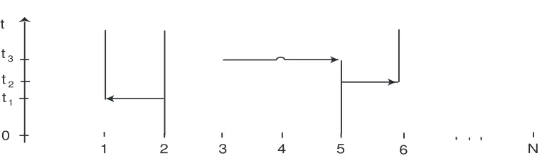
with rate parameterλk. At every time point of this Poisson process, the configuration of (i, j) changes according to fk. For example, if the pair of types was (1,0) before, then it changes tofk(1,0)∈ {0,1}2. All Poisson processes are supposed to be independent. This construction
can be visualised by drawing arrows from i to j at the time points of the Poisson processes associated with the pair (i, j) (cf. Figure 1).
As an example, consider the following continuous timeMoran model (MN
t )t≥0with state space
{0,1}N. This is a population genetic model where ordered pairs of individuals resample at rateβ/N,β >0. When a resampling event occurs at (i, j), individualibequeaths its type to individualj. Thus, the basic mechanism isfR defined by
fR(1,·) := (1,1), fR(0,·) := (0,0). (8)
Figure 1 shows a realisation with three resampling events. At timet1, the pair (2,1) resamples.
The arrow in Figure 1 at time t1 indicates that individual 2 bequeaths its type to individual
1. Furthermore, individual 5 inherits the type of individual 3 at time t3. The dual process of
the Moran model is a coalescent process. This process is defined by the coalescent mechanism
fC given by
fC(1,·) := (0,1), fC(z) :=z, z∈ {(0,0),(0,1)}, (9)
N 6
5 4
3 2
1 0
t t
1 3
t
2
Figure 1: Three resampling events. Type 1 is indicated by black lines, absent lines correspond to type 0.
fR and fC are dual, and why this implies (5) (see Proposition 2.3). More generally, we will identify all dual pairs of basic mechanisms.
Our method elucidates the role of the square in (3) for the duality of the logistic Feller diffusion with another logistic Feller diffusion. We illustrate this by the Laplace duality of Feller’s branching diffusion (Ft)t≥0, which is the logistic Feller diffusion with parameters (0,0, β), β >0. Its dual process (yt)t≥0 is the logistic Feller diffusion with parameters (0, β,0), i.e., the
solution of the ordinary differential equation
d
dtyt=−β y 2
t, y0=y∈[0,∞). (10)
The duality relation between these two processes isEx[e−Fty] =e−xyt,t≥0. In Theorem 4.3,
we prove that the rescaled Moran model |MN t√N|/
√
N
t≥0 converges weakly to (Ft)t≥0 as N → ∞. To get an intuition for this convergence, notice that (|MN
t |)t≥0is a pure birth-death
process with size-dependent transition rates (“birth” corresponds to creation of an individual with type 1, whereas “death” corresponds to creation of an individual with type 0). It remains to prove that the birth and death events become asymptotically independent asN → ∞. It is known, see e.g. Section 2 in [3], that the dual process of the Moran model (MN
t )t≥0,N ≥1,
is a coalescing random walk. Furthermore, the total number of particles of this coalescing random walk is a pure death process on{1, ..., N}which jumps fromktok−1 at exponential rate Nβk(k−1), 2 ≤k≤ N. This rate is essentially quadratic in k for large k. We will see that a suitably rescaled pure death process converges to a solution of (10); see Remark 4.5. The square in (10) originates in the quadratic rate of the involved pure death process; see the equations (42) and (29) for details.
In the literature, e.g. [9], the duality function H(xN, yN) =
1
xN
≤yN, xN, yN ∈ {0,1}N, can
be found frequently, wherexN ≤yN denotes component-wise comparison. Processes (XN t )t≥0
and (YN
t )t≥0 with state space{0,1}N are dual with respect to this duality function if they
satisfy
PxN
XtN ≤yN
=PyN
xN ≤YtN
∀xN, yN ∈ {0,1}N, t≥0. (11)
The biased voter model is dual to a coalescing branching random walk in this sense (see [8]). Property (11) could also be used to derive the dualities mentioned in this introduction. In fact, the two properties (5) and (11) are equivalent in the following sense: If (XN
t )t≥0 and (YtN)t≥0
satisfy (5) then (XN
t )t≥0 and (1−YtN)t≥0 satisfy (11) and vice versa. In the configuration
of the process (1−YN
t )t≥0 is easily obtained from the dynamics of (YtN)t≥0 by interchanging
the roles of the types 0 and 1.
2
Dual basic mechanisms
Fix m ∈ N and let (X
N
t )t≥0 and (YtN)t≥0 be two processes defined by basic mechanisms
(f1, ..., fm) and (g1, ..., gm), respectively. Suppose that the Poisson processes associated with k≤mhave the same rate parameterλk ≥0,k= 1, . . . , m. We introduce a property of basic mechanisms which will imply (5).
Definition 2.1 Let f, g :{0,1}2 → {0,1}2 and for x= (x
1, x2)∈ {0,1}2 let x† := (x2, x1).
The basic mechanisms f andg are said to bedualiff the following two conditions hold: ∀x, y∈ {0,1}2: y∧ f(x)†
= (0,0) =⇒ g(y)∧x† = (0,0), (12)
∀x, y ∈ {0,1}2: x∧ g(y)†
= (0,0) =⇒ f(x)∧y† = (0,0). (13)
To see how this connects to the duality relation in (5), we illustrate this definition by an example.
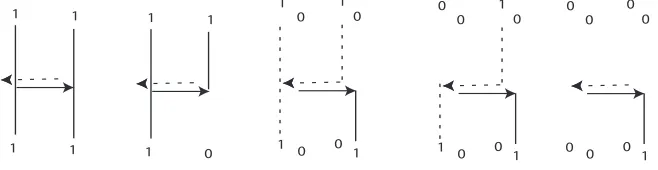
Example 2.2 The resampling mechanism fR defined in (8) and the coalescent mechanism
fC defined in (9) are dual. We check condition (12) with f = fR and g = fC by looking at Figure 2. The resampling mechanism acts in upward time (solid lines), the coalescent
1 0
1 1
1 1
1 1
0 1
0 0
1 1
1 0
0 1
0 0
0 1
1 0
0 1
0 0
0 0
0 0
Figure 2: The resampling mechanism and the coalescent mechanism satisfy (12)
mechanism in downward time (dashed lines). There are three nontrivial configurations forx, i.e., (1,1), (1,0) and (0,1). In the first two cases, we havefR(x) = (1,1). Then onlyy= (0,0) satisfies y ∧(fR(x))† = (0,0). In the third case, every y satisfies y ∧(fR(0,1))† = (0,0) and has to be checked separately. We see that whenever the configuration y is disjoint from (f(x))†, i.e.,y∧(f(x))†= (0,0), theng(y) is disjoint fromx†. The coalescent mechanism is the
0 0 0 0
1 0 0
1 0 0
1 0
0 1/0
0 0
1 0 0
1/0 0 0
1 0
? ?
? ?
0 0
Figure 3: The resampling mechanism and the coalescent mechanism satisfy (13)
The following proposition shows that two processes are dual in the sense of (5) if their defin-ing basic mechanisms are dual (cf. Definition 2.1). The proofs of both Proposition 2.3 and Proposition 3.1 follow similar ideas as in [5].
Proposition 2.3 Let m∈Nand let the processes (X
N
t )t≥0 and(YtN)t≥0 be defined by basic
mechanisms(f1, ..., fm)and(g1, ...,gm), respectively. Suppose that the Poisson processes
asso-ciated withk∈ {1, . . . , m} in(XN
t )t≥0 and in(YtN)t≥0 have the same rate parameter λk ≥0. If fk and gk are dual for everyk = 1, . . . , m, then (XtN)t≥0 and (YtN)t≥0 satisfy the duality
relation (5).
Proof: FixT >0 and initial valuesXN
0 , Y0N ∈ {0,1}N. Assume for simplicity thatm= 1
and letf :=f1,g:=g1. Define the process ˆYtN
0≤t≤T in backward time in the following way. Reverse all arrows in the graphical representation of (XN
t )t≥0. At (forward) timeT, start with
a type configuration given by ˆYN
0 :=Y0N. Now proceed until (forward) time 0: Whenever you
encounter an arrow, change the configuration according tog. Recall that the direction of the arrow indicates the order of the involved individuals. We show that the processes (XN
t )t≥0
and ( ˆYN
t )0≤t≤T satisfy
X0N∧YˆTN = 0 ⇐⇒ XTN ∧Yˆ0N = 0 ∀X0N,Yˆ0N ∈ {0,1}N, (14)
for every realisation. We prove the implication “ =⇒” by contradiction. Hence, assume that for some initial configuration there is a (random) timet∈[0, T] such that
X0N∧YˆTN = 0 and XtN ∧YˆTN−t6= 0. (15)
There are only finitely many arrows until time T and no two arrows occur at the same time almost surely. Hence, there is a first time τ such that the processes are disjoint before this time but not after this time. The arrow at timeτpoints fromitoj, say. Denote by (x−i , x−j)∈ {0,1}2and (x+
i , x
+
j) the types of the pair (i, j)∈ {1, ..., N}2according to the process (XtN)t≥0
immediately before and after forward timeτ, respectively. By the definition of the process, we then havef(x−i , x−j ) = (x+i , x+j). Furthermore, denote by (yj−, y−i ) the types of the pair (j, i) according to (YN
t )t≥0 immediately before backward timeT −τ. We have chosenτ, i, j such
that
(x−i , x−j)∧ g(y−j, yi−)†
= (0,0) and (x+i , x+j)∧(y−i , yj−)6= (0,0). (16)
It remains to prove that YN
T and ˆYTN are equal in distribution. The assertion then follows from
P
X0N ∧YTN = 0
=P
X0N ∧YˆTN = 0
(14)
= P
XTN ∧Yˆ0N = 0
=P
XTN∧Y0N = 0
. (17)
If a Poisson process is conditioned on its value at some fixed time T >0, then the time points are uniformly distributed over the interval [0, T]. The uniform distribution is invariant under time reversal. In addition, the Poisson processes of (YN
t )t≥0 nd (XtN)t≥0 have the same rate
parameter. Thus, (YN
t )0≤t≤T and ( ˆYtN)0≤t≤T have the same one-dimensional distributions. ✷
We will now give a list of those maps f :{0,1}2→ {0,1}2 for which there exists a dual basic
mechanism (see Definition 2.1). The mapsf andgin every row of the following table are dual to each other. As in Example 2.2, it is elementary to check this.
No f(0,0) f(0,1) f(1,0) f(1,1) g(0,0) g(0,1) g(1,0) g(1,1) i) (0,0) (0,0) (1,1) (1,1) (0,0) (0,1) (0,1) (0,1) ii) (0,0) (0,1) (1,1) (1,1) (0,0) (0,1) (1,1) (1,1) iii) (0,0) (0,0) (0,1) (0,1) (0,0) (0,0) (0,1) (0,1) iv) (0,0) (0,1) (1,0) (1,1) (0,0) (0,1) (1,0) (1,1) v) (0,0) (1,1) (1,1) (1,1) (0,0) (1,1) (1,1) (1,1) vi) (0,0) (0,0) (0,0) (0,0) (0,0) (0,0) (0,0) (0,0)
Check that the pair (f, g) is dual if and only if the pair (f†, g†) is dual wheref†(x) := (f(x†))†.
Furthermore, the pair (f, g) is dual if and only if ( ˆf ,ˆg†) is dual where ˆf(x) := f(x†) and
ˆ
g†(x) = (g(x))† forx∈ {0,1}2. Thus, for each of the listed dual pairs (f, g), the pairs (f†, g†),
( ˆf ,ˆg†) and ( ˆf†,gˆ) are also dual. Modulo this relation, the listing of dual basic mechanisms is
complete. The proof of this assertion is elementary but somewhat tedious and is thus omitted. Readers interested in the proof are invited to contact the authors in order to get the detailed classification of dual basic mechanisms.
Of particular interest are the dualities in i)-iii). The first of these is the duality between the resampling mechanism and the coalescent mechanism, which we already encountered in Example 2.2. The duality in ii) is the self-duality of thepure birth mechanism
fB :{0,1}2→ {0,1}2,(1,0)7→(1,1) andx7→x∀x∈ {(0,0),(0,1),(1,1)} (18)
and iii) is the self-duality of the death/coalescent mechanism
fDC:{0,1}2→ {0,1}2,(1,·)7→(0,1) and (0,·)7→(0,0). (19)
We are only interested in the effect of a basic mechanism on the total number of individuals of type 1. The identity map in iv) does not change the number of individuals of type 1 in the configuration. The effect of v) and vi) on the number of individuals of type 1 is similar to the effect of ii) and iii), respectively. Furthermore, bothf† and ˆf have the same effect on the
number of individuals of type 1 asf.
Closing this section, we define processes which satisfy the duality relation (5). These processes will play a major role in deriving the dualities (2) and (4) in Section 4. For u, e, γ, β≥0, let (XN
t )t≥0= (XtN,(u,e,γ,β))t≥0 be the process on{0,1}N with the following transition rates (of
N
• With rate Ne, the death/coalescent mechanismfDC occurs (cf. (19)).
• With rate Nγ, the coalescent mechanismfC occurs (cf. (9)).
• With rate Nβ, the resampling mechanismfR occurs (cf. (9)).
Together with an initial configuration, this defines the process. The process (XtN,(u,e,γ,β))t≥0
is defined by the basic mechanisms (fB, fDC, fC, fR), and the process (XN,(u,e,β,γ)
t )t≥0 is
defined by the basic mechanisms (fB, fDC, fR, fC). Proposition 2.3 then yields the following corollary.
Corollary 2.4 Let u, e, γ, β ≥ 0. The two processes (XtN,(u,e,γ,β))t≥0 and (XtN,(u,e,β,γ))t≥0
satisfy the duality relation (5).
3
Prototype duality
In this section, we derive the prototype duality (6) from (5). The main idea for this is to integrate equation (5) in the variablesxN and yN with respect to a suitable measure. Fur-thermore, we will exploit the fact that drawing from an urn with replacement and without replacement, respectively, is almost surely the same if the urn contains infinitely many balls.
Proposition 3.1 Let (XN
t )t≥0 and (YtN)t≥0 be processes with state space {0,1}N, N ≥ 1.
Assume that (XN
t )t≥0 and (YtN)t≥0 satisfy the duality relation (5). Choose n, k ∈ {0, ..., N}
which may depend on N. Define µNn(xN) := N
n
−1
1
|xN
|=n for every xN ∈ {0,1}N where |xN| = PN
i=1xNi is the total number of individuals of type 1. Assume L X0N
= µN n and L YN
0
=µN
k. Suppose that the process(XtN)t≥0 satisfies n
N →0 and
E XtNN
N −→0 asN → ∞, (20)
wheretN ≥0. Then
lim N→∞E
"
1−Nk
XtNN
#
= lim N→∞E
"
1−
YtNN
N
n #
(21)
under the assumption that the limits exist.
Proof: A central idea of the proof is to make use of the well known fact that the hyper-geometric distribution Hyp(N, R, l), R, l ∈ {0, ..., N}, can be approximated by the binomial distribution B(l,R
N) asN → ∞provided that l is sufficiently small compared to N. In fact, by Theorem 4 of [2],
B(l,
R N)
{0}
−Hyp(N, R, l)
{0} ≤dT V
B l,NR
,Hyp(N, R, l)
≤4N·l ∀R, l≤N,
where dT V is the total variation distance. By assumption (20), we have (withR := k, l :=
as N → ∞. By definition of the hypergeometric distribution, we get
Hyp N,
By the same argument, we also obtain
Hyp N, k,
t )t≥0 started in the fixed initial configuration xN ∈ {0,1}N. Starting from the left-hand side of (21), the above considerations yield
Eh 1− k
which proves the assertion. ✷
4
Various scalings
Recall the definition of the process (XtN,(u,e,γ,β))t≥0from the end of Section 2. DefineXtN :=
XtN,(u,e,γ,β) and YtN := X
N,(u,e,β,γ)
t fort ≥0 and N ∈ N. Notice that the Poisson process
attached to the resampling mechanism in the process (YN
t )t≥0 has rate γ. By Corollary 2.4,
≥ ≥
process and the(1, b, c, d)-resem-process, respectively. The initial values areX0=n∈N0 and
Y0=y∈[0,1]. Then
En
(1−y)Xt=Ey(1
−Yt)n
, t≥0. (28)
Remark 4.2 In the special case b = 0 = d and c > 0, this is the moment duality of the Fisher-Wright diffusion with Kingman’s coalescent. Furthermore, choosingc= 0 andb, d >0 results in the moment duality of the Galton-Watson process with a deterministic process.
Proof: Choose u, e, β ≥0 and γ =γ(N) such that b = u+β, d =e+β and γ/N → c
as N → ∞. In the first step, we prove that the process (|XN
t |)t≥0 of the total number of
individuals of type 1 converges weakly to (Xt)t≥0. The total number of individuals of type
1 increases by one if a “birth event” occurs (fB or fR) and if the type configuration of the respective ordered pair of individuals is (1,0). If the total number of individuals of type 1 is equal tok, then the probability of the type configuration of a randomly chosen ordered pair to be (1,0) is Nk NN−−k1. The number of Poisson processes associated with a fixed basic mechanism isN(N−1). Thus, the process of the total number of individuals of type 1 has the following transition rates:
k→k+ 1 : u+Nβ·N(N−1)· k N
N−k N−1, k→k−1 : e+Nβ ·N(N−1)·NN−k
k N−1+
e+γ
N ·N(N−1)· k N
k−1
N−1,
(29)
where k ∈N0. Notice that the coalescent mechanism produces the quadratic term k(k−1)
because the probability of the type configuration of a randomly chosen ordered pair to be (1,1) is k
N k−1
N−1 if there are k individuals of type 1. The transition rates determine the generator
GN =GN,(u,e,γ,β)of (|XN
t |)t≥0, namely
GNf(k) =u+β
N ·k(N−k)· f(k+ 1)−f(k)
+e+β
N ·k(N−k)· f(k−1)−f(k)
+e+γ
N ·k(k−1)· f(k−1)−f(k)
, k∈ {0, . . . , N},
(30)
forf:{0, . . . , N} →R. The (1, u+β, c, e+β)-braco-process (Xt)t
≥0is the unique solution of
the martingale problem forG (see [1]) where
Gf(k) := (u+β)k f(k+ 1)−f(k)
+ (e+β) +c(k−1)
k f(k−1)−f(k)
, k∈N0,
(31) forf: N0→Rwith finite support. LettingN → ∞, we see that
GNf(k)−→ Gf(k) as N→ ∞, k∈N0, (32)
forf:N0 →Rwith finite support. We aim at using Lemma 5.1 which is given below (with
EN ={0, . . . , N}andE=N0), to infer from (30) the weak convergence of the corresponding
Markov processes. A coupling argument shows that (|XN
t |)t≥0 is dominated by (ZtN)t≥0 :=
(|XtN,(u,0,0,β)|)t≥0. The process (ZtN)t≥0 solves the martingale problem forGN,(u,0,0,β). Thus,
we obtain
ZtN −Z0N =
Z t
0 G
N,(u,0,0,β)ZN
s ds+CtN =
Z t
0 uZsN
N−ZN s
N ds+C N
where (CN
t )t≥0 is a martingale. Hence, (ZtN)t≥0 is a submartingale. Taking expectations,
Gronwall’s inequality implies
E[ZtN]≤E[Z0N]eut, ∀t≥0. (34)
LetSN =TN = 1, sN =uand recall|X0N|=n. With this, the assumptions of Lemma 5.1 are
satisfied. Thus, Lemma 5.1 implies that (|XN
t |)t≥0 converges weakly to (Xt)t≥0 as N → ∞.
variables with complete and separable state space converges weakly to ˜X and if the sequence (fn)n∈N,fn∈Cb, converges uniformly on compact sets tof ∈Cb, thenE[fn( ˜Xn)]→E[f( ˜X)]
The next step is to prove that the rescaled processes (|YN
t |/N)t≥0 converge weakly to (Yt)t≥0 Lemma 5.1 are satisfied and we conclude that (|YN
t |/N)t≥0 converges weakly to (Yt)t≥0. It
imply condition (20). Thus, Proposition 3.1 establishes equation (21). The assertion follows
from equations (35), (21) and (39). ✷
≥
For β, γ > 0 and r = γ/β, Theorem 4.3 yields the self-duality of the logistic Feller diffusion. prove that the rescaled process (|YN
t√N|/(r √
N))t≥0 converges weakly to (Yt)t≥0 as N → ∞.
The generator of the rescaled process is given by (cf. (36))
√
c([0,∞)). Notice that the quadratic termy2 originates in the quadratic term
k(k−1). Hutzenthaler and Wakolbinger [7] prove that (Yt)t≥0 is the unique solution of the
martingale problem for G. Let |YN
which dominates (YN
t )t≥0 and which satisfies of Lemma 5.1 are satisfied and we conclude that (|YN
uniformly in 0≤z ≤z˜. Together with the weak convergence of the rescaled processes, this
N. Inequality (43) and |XN
0 |=n << N imply condition (20). Thus, Proposition 3.1 establishes equation (21). The
assertion follows from equations (45), (21) and (46). ✷
Remark 4.5 Assume u = e = γ = α = 0 and r = 1 in the proof of Theorem 4.3. Then (|YN
t |)t≥0 is a pure death process on{1, ..., N} which jumps fromk to k−1 at exponential
rate Nβk(k−1), 2≤k≤N. Furthermore, (Yt)t≥0 is a solution of (10). We have just shown
that the rescaled pure death process (|YN t√N|/
√
N)
t≥0converges weakly to (Yt)t≥0asN → ∞.
5
Weak convergence of processes
In the proofs of Theorem 4.1 and Theorem 4.3, we have established convergence of generators plus a domination principle. In this section, we prove that this implies weak convergence of the corresponding processes. For the weak convergence of processes with c`adl`ag paths, let the topology on the set of c`adl`ag paths be given by the Skorohod topology (see [4], Section 3.5).
Lemma 5.1 Let E ⊂R
Proof: We aim at applying Corollary 4.8.16 of Ethier and Kurtz [4]. For this, define
t≥0
has state space ˜EN and generator ˜GN. Now we prove the compact containment condition, i.e., for fixedε, t >0 we show
∃K >0
∀N ∈N
Phsup s≤t
YsTNN SN ≤
Ki≥1−ε. (50)
UsingYN
t ≤ZtN,t≥0, and Doob’s Submartingale Inequality, we conclude for allN ∈N
Phsup s≤t
YsTNN ≥KSN
i
≤Phsup s≤t
ZsTNN ≥KSN
i
≤ KS1 N
E
ZtTNN
≤ K1 sup N∈N
E
ZN
0
SN ·
exp t· sup N∈N
(sNTN)=:
C K.
(51)
Thus, choosingK:=C
ε completes the proof of the compact containment condition.
It remains to verify condition (f) of Corollary 4.8.7 of [4]. Condition (47) implies that for every
f ∈C2
c and every compact setK⊂E
sup y∈K∩E˜N
|G˜Nf(y)− Gf(y)| →0 asN → ∞. (52)
Choose a sequence KN such that (52) still holds with K replaced by KN. This together with the compact containment condition implies condition (f) of Corollary 4.8.7 of [4] with
GN :=KN∩E˜N andfN :=f|E˜N. Furthermore, notice thatC 2
c(E) is an algebra that separates points andE is complete and separable. Now Corollary 4.8.16 of Ethier and Kurtz [4] implies
the assertion. ✷
Open Question:
Athreya and Swart [1] prove a self-duality of the resem-process given by (1). We were not able to establish a graphical representation for this duality. Thus, the question whether our technique also works in this case yet waits to be answered.Acknowledgements:
We thank Achim Klenke and Anton Wakolbinger for valuable dis-cussions and many detailed remarks. Also, we thank the referee for a number of very helpful suggestions.References
[1] Athreya, S. R. and Swart, J. M.(2005). Branching-coalescing particle systems.Probab. Theory Related Fields 131, 3, 376–414. MR2123250
[2] Diaconis, P. and Freedman, D. A. (1980). Finite exchangeable sequences. Ann. Probab.8, 4, 745–764. MR0577313
[3] Donnelly, P.(1984). The transient behavior of the Moran model in population genetics. Math. Proc. Cambridge Philos. Soc.95, 2, 349–358. MR0735377
[5] Griffeath, D. (1979). Additive and cancellative interacting particle systems. Lecture Notes in Mathematics, Vol. 724. Springer, Berlin. MR0538077
[6] Harris, T. E.(1978). Additive set-valued Markov processes and graphical methods.Ann. Probability 6, 3, 355–378. MR0488377
[7] Hutzenthaler, M. and Wakolbinger, A.(2007). Ergodic behavior of locally regulated branching populations. Ann. Appl. Probab.17, 2, 474–501. MR2308333
[8] Krone, S. M. and Neuhauser, C. (1997). Ancestral processes with selection. Theor. Popul. Biol.51, 3, 210–237.