T H E J O U R N A L O F H U M A N R E S O U R C E S • 46 • 4
Does Schooling Lead to an Extended Old
Age?
Hans van Kippersluis
Owen O’Donnell
Eddy van Doorslaer
A B S T R A C T
While there is no doubt that health is strongly correlated with education, whether schooling exerts a causal impact on health is not firmly estab-lished. We exploit a Dutch compulsory schooling law to estimate the causal effect of education on mortality. The reform provides a powerful in-strument, significantly raising years of schooling, which, in turn, has a sig-nificant and robust negative effect on mortality. For men surviving to age 81, an extra year of schooling is estimated to reduce the probability of dy-ing before the age of 89 by almost three percentage points relative to a baseline of 50 percent.
I. Introduction
Inequalities in health and life expectancy by education are striking. In the Netherlands, individuals with a university or college degree live, on average,
Hans van Kippersluis is assistant professor of applied economics at Erasmus University Rotterdam (the Netherlands). Owen O’Donnell is an associate professor of applied economics at the University of Mac-edonia (Greece) and Erasmus University Rotterdam (the Netherlands). Eddy van Doorslaer is a profes-sor of health economics at the Erasmus School of Economics and the Institute for Health Policy and Management of the Erasmus University in Rotterdam (the Netherlands). The authors thank Netspar (pro-ject “Health and Income, Work and Care across the Life Cycle II”), and the National Institute of Aging (R01AG037398–01) for financial support. The authors acknowledge access to linked data resources (RIO 1998, POLS Basis 1997–2005, and DO 1998–2005) by the Netherlands Central Bureau of Statistics (CBS). Further they thank Maarten Lindeboom, Frank Windmeijer, Paul Devereux, Daniele Fabbri, Mar-loes Lammers, Pilar Garcia-Gomez, Tom Van Ourti, Esen Erdogan-Ciftci, Teresa Bago d’Uva, the anon-ymous referees, and seminar participants of the Empirical Health Economics—Ifo / CESifo & University of Munich conference, iHEA World Congress in Beijing, University of Lausanne, Netspar Pension Days, Tinbergen Institute, and Erasmus University Rotterdam for helpful comments. Researchers hoping to use the data found in this article can apply for access to the Netherlands Central Bureau of Statistics (CBS). The authors of this paper are willing to offer guidance about the application.
[Submitted March 2010; accepted October 2010]
six to seven years longer than those who finished only primary school. The difference in life expectancy in good health is as much as 16 to 19 years (CBS 2008). Such disparities in health and mortality by education have been documented for many countries (Grossman and Kaestner 1997; Smith and Kington 1997; Mackenbach et al. 2008; Cutler and Lleras-Muney 2008). Yet, very few studies have found robust evidence of a causal impact of education on health. The correlation also could stem from childhood ill-health constraining educational attainment (Perri 1984; Behrman and Rosenzweig 2004; Case, Fertig, and Paxson 2005) and confounding factors such as ability and time preference (Fuchs 1982; Berger and Leigh 1989; Auld and Sidhu 2005; Deary 2008). Establishing whether education causally impacts on health is essential to the formation and evaluation of education and health policies.
The purpose of this paper is to establish whether education has a causal impact on mortality in old age using exogenous variation in education that comes from a compulsory schooling law introduced in the Netherlands in 1928. This reform, which increased the educational attainment of the population suddenly and strongly, pro-vides a valuable instrument within a regression discontinuity design. We directly observe deaths in a very large sample of individuals tracked between the ages of 81 and 89. This makes it possible to investigate whether there are long-run health returns to education that accumulate and result in an extended life.
Lleras-Muney (2005; 2006), exploiting changes in compulsory schooling and child labor laws in more than 30 U.S. states, estimates that an additional year of schooling reduces the ten-year probability of dying by at least 3.6 percentage points. This analysis is based on only an approximation to mortality derived from the change in cohort size between subsequent censuses and Mazumder (2008) demonstrates that the magnitude and the significance of the effect are not robust to allowing mortality trends around the affected cohorts to differ across states possibly due to differences in public health measures. Clark and Royer (2010), who measure mortality somewhat more directly than Lleras-Muney (2005), find that the 1947 and 1972 extensions to the school leaving age in the United Kingdom had strong impacts on educational attainment, but no significant effects on mortality. Albouy and Lequien (2009) ex-ploit two compulsory schooling reforms in France in 1923 and 1953. They do not find a significant effect of education on mortality, which is observed directly from micro data, possibly because the reforms did not have very strong impacts on years of schooling.
While the weight of existing evidence does not support an effect of education on mortality (Mazumder 2008; Albouy and Lequien 2009; Clark and Royer 2010), some (but not all) studies using compulsory schooling laws as a source of exogenous variation in education find an effect on self reported health outcomes (Spasojevic 2003; Oreopoulos 2006; Mazumder 2008; Silles 2009) and hospitalizations (Arendt 2008). An obvious weakness of evidence based on self-reported health is that re-porting thresholds may vary with education (Bago d’Uva, O’Donnell, and Van Doorslaer 2008). If this is the case, the resulting bias would not be corrected by instrumenting education.1
The main weakness of most of the analyses of mortality, with the notable excep-tion of Albouy and Lequien (2009), is that they rely on approximate measures of mortality at the cohort level rather than directly observed survival at the individual level. We observe a very large number of individuals from linked Dutch adminis-trative and survey data for which a mortality followup is available. Given the strong instrument, provided by the compulsory schooling reform, and tremendous power, generated by the sample size and micro data, it is quite unlikely that we will fail to detect an effect of education on mortality should one exist in the population.
We find that education significantly lowers mortality in old age. For men surviving to 81, an additional year of schooling reduces the probability of dying before reach-ing 89 by almost three percentage points, relative to a baseline probability of 50 percent. Increased education generates health returns that accumulate and are main-tained over the long run—possibly by permanently improving health behavior, re-ducing occupational risks, raising income or endowing ability to manage chronic diseases—and become manifest in improved survival chances at an advanced age. Our estimate of a 6 percent reduction in the eight-year probability of death at age 81 is not necessarily indicative of the magnitude of any effect operating at other ages. But provided education does not reduce the probability of survival to 81, then, within the Dutch context, we can conclude that observed differences in life expec-tancy by education in early adulthood are, at least in part, attributable to a causal effect of education.
A significant impact is found only with the larger of our samples, which is con-sistent with lack of statistical power partly explaining why most previous studies have found no evidence of a causal impact of education on mortality. The strength of our compulsory schooling law instrument, the fact that this took effect at a rela-tively low level of education, inducing children to enter secondary school, and the advanced age of our sample, which ensures both that health returns to education are fully accumulated and mortality rates are high, would also seem to be important contributors to finding a significant effect.
The paper is organized as follows. Section II provides background information on the Dutch reforms that enable us to estimate the causal impact of education on mortality. The data and methods are discussed in Section III. The main results are presented in Section IV. The concluding section considers explanations for discrep-ancies between our findings and those of other studies and acknowledges limitations of the present study.
II. Compulsory Schooling Laws in the Netherlands
(Idenburg 1964, p. 489). Since after 1920 entry during the year was no longer allowed in most cases, more and more children entered school between the ages of five and one half and six (Sterringa 1934, p. 88).
Lack of resources meant that the 1922 law was never enforced (Hentzen 1932). In 1924, the number of years of compulsory schooling was officially reversed from 7 to 6 and the increase postponed until 1930. But an improvement in the economy prompted the government, in response to a request from parliament, to bring the rise forward to July 1st 1928 (Hentzen 1932; De Graaf 2000). The law had an effect at the transition of the school year (Hentzen 1932, p. 185) and so came fully into effect for all schools only at the start of the new school year (CBS 1931, p. 19; Mandemakers 1996, p. 55), which was August/September in cities and March/April in the countryside (CBS 1931, p. 36). Consequently, the law was only universally enforced from the year 1929 onward (CBS 1931, p. 19; Mandemakers 1996, p. 55). On 24 June 1929 (Staatsblad 1929), the law was rephrased to clarify that children attending a school with only six grades had to complete a seventh year at another school (Hentzen 1932, p. 206; Sterringa 1934, p. 96). Before that date, some parents registered their child at a six-grade school to circumvent the seventh compulsory year of schooling (Gielen 1984, p. 124). Because most primary schools had only six grades, the reform induced—as we will show later—a large proportion of pupils to enter and complete secondary school.
Individuals born in 1916, who started school at age six, or younger, would have fulfilled their schooling obligations under the old regime before the new law was enforced (Sterringa 1934, p. 113). This cohort was not affected by the reform. In-dividuals born in 1917 were at most 11 on July 1, 1928, and could not have met the conditions to leave school under the pre-1928 legal regime. The cohort born in 1917 was the first to be affected by the 1928 reform and to be forced to complete seven, rather than six, years of schooling. Therefore, we put the reform threshold at a birth date of January 1, 1917.2
Compulsory schooling was raised further to eight years in 1942 under the German occupation with the aim of promoting the German language. A lack of competent teachers and materials, and resistance from the population, meant that both the qual-ity of the extra education and compliance with the law were very low (Meijsen 1976; HSG 1946/1947).3 After the war, a new law confirmed the increase in the
minimum years of schooling to eight, but deferred its enforcement to January 1, 1950 given high rates of school absence and the unpopularity of the war-time in-crease, circumvention of which had become almost a heroic deed (HTK 1946/1947).4
We have confirmed that the 1950 reform did induce some individuals to obtain more
2. It is possible that some individuals born in 1916 who started school at age seven were affected by the reform, and some individuals born in 1917 who started school at age 5 were allowed to drop out. But these cases are plausibly small fractions of the total. We do not observe place of birth and so cannot distinguish between rural and urban residents who started school in April and September respectively. It is not therefore possible to determine the reform threshold with 100 percent accuracy for every observation. But this is not vital in a Fuzzy Regression Discontinuity Design (RDD) since the only requirement is that the probability of receiving treatment jumps discontinuously at the threshold, which, as we will show later, is obviously the case in our application.
schooling, but the effect is not large and so does not provide a strong instrument for education. Later increases in the minimum school leaving age in 1969, 1975, and 1985 also do not provide clear first-stage discontinuities and given the very low mortality rates observed in individuals below the age of 40, it is likely that even the large sample available for this study would be insufficient to detect small effects. In the analysis we restrict attention to the 1928 reform, which, as will become apparent, had a strong impact on educational attainment.
III. Data and Methods
A. Data
Our data are linked survey and administrative records from Statistics Netherlands. We use the annual cross-sectional general household survey (POLS) 1997–2005, the tax records (RIO) for 1998, and the Cause-of-Death register for 1998 until 2005 inclusive. All these files are linked to the Dutch Municipality Register (GBA), which covers, among others, date of birth, sex, province, and ethnicity.
The POLS samples a representative cross-section of the noninstitutionalized Dutch population ranging from around 10,000 to 80,000 respondents per year.5It collects
extensive information on demographic and socioeconomic characteristics. The re-spondent’s education is recorded by two variables: the highest level followed and that finished on the standard Dutch categorization [Standaard Onderwijs Indeling (SOI) 1998].6The SOI is very close to the International Classification of Education
(ISCED) and is easily converted into years of schooling following standard guide-lines (SHARE 2007).7In the relatively few cases that individuals reported to have
followed a higher level than they finished, we take the average of the corresponding years.8 Through linkage with the Cause-of-Death register we are able to observe
death and its cause for all POLS respondents who died between 1998 and 2005. The RIO is a huge administrative tax-register covering one third of the Dutch population, around five million observations per year. Apart from detailed income information, it also contains demographics. By linking the RIO tax records to the Cause-of-Death register we observe, again, mortality for all individuals. Unfortu-nately, education information is not available in the RIO, but, as will be explained below, it is still possible to combine estimates from the linked RIO-death register
5. Specifically 34,439 in 1997, 80,789 in 1998, 42,605 in 1999, 37,482 in 2000, 24,231 in 2001, 22,259 in 2002, 25,163 in 2003, 21,706 in 2004, and 10,378 in 2005.
6. SOI is missing in the 2003 wave of the POLS. However, there is a highly similar educational variable available in that year, which is redefined into SOI and ISCED.
7. The Dutch SOI consists of seven levels of education: toddler school, primary education (six years), lower vocational secondary education (ten years), higher general secondary education (13 years, similar to high school), first phase higher education (15 years, intermediary vocational education), second phase higher education (16 years, higher vocational education) and third phase higher education (17 years, uni-versity education).
with those from the POLS to obtain instrumental variable (IV) estimates of the impact of education on mortality.
The CBS Linked Data are unique in the context of data that have been used previously to estimate the impact of education on health in the sense that they provide a mortality followup of both a sample survey (POLS, 1997–2005) and a very large administrative database (RIO, 1998). So, individual mortality is observed, and with the POLS we observe both education and mortality for the same sample observations. The mortality record provides eight years of followup by cause of death. Given that the cohorts affected by the reform we study were born after 1916, we observe these individuals in their 80s9and cannot estimate any impact that
edu-cation has on survival to 81.10We estimate the effect of years of schooling on the
probability of dying between 81 and 88 (inclusive), conditional on being alive at age 81. If education raises the probability of survival to 81, then this presample selective mortality will downwardly bias our estimate of the impact on the condi-tional probability. Low-educated individuals who manage to survive to 81 must be atypically robust in their health relative to the population of low-educated individuals in the same birth cohort. Highly educated individuals surviving to 81 do so, assuming there is an education effect, in part, because of, rather than in spite of, their edu-cation.11Consequently, highly educated survivors will not have such strong inherent
health as their low-educated counterparts. Any positive effect of education on sur-vival beyond 81 will have to overcome these unobservable health differences be-tween low and highly educated survivors to 81 and so the estimate of the causal effect will be biased downward. Note that the bias will not be corrected by our IV estimator—the unobservable differences would exist in the surviving sample even if education were allocated randomly. But, if education does indeed raise the prob-ability of survival to 81, then at least we know that we will identify a lower bound on the true causal effect of education on mortality between 81 and 89.
B. Identification Strategy and Estimation
We exploit the 1928 compulsory schooling law as an instrument for education within the framework of a Regression Discontinuity Design (RDD) (Thistlethwaite and Campbell 1960; Trochim 1984; Hahn, Todd, and Van der Klaauw 2001; Lee and Card 2008; Imbens and Lemieux 2008; Van der Klaauw 2008; Lee and Lemieux 2010). All analyses are done separately for males and females. Year of birth (cohort) determines whether the individual is exposed to the reform, so sorting around the threshold is absent. Furthermore, not all individuals exposed to the reform are
in-9. An estimated 25 percent of Dutch males born in 1917 and 49 percent of females is still alive at age 81 and, for this cohort, life expectancy at birth was around 60 for males and 68 for females [Human Mortality Database,University of California, Berkeley (USA), and Max Planck Institute for Demographic Research (Germany) www.mortality.org].
10. Physical censuses have been abolished in the Netherlands since 1991, with 1971 being the last available one. In 2001, there was a “virtual” census based on administrative data. The absence of recent, comparable census data makes it difficult to estimate cohort mortality rates indirectly and to use these to estimate the impact of education on survival to age 81.
duced by it to change their education. We therefore have a discrete running-variable Fuzzy Regression Discontinuity setup (Lee and Card 2008) and the appropriate es-timator is parametric Two Stage Least Squares (2SLS), in which years of education is instrumented by the reform. Under the standard assumptions of RDD (Hahn, Todd, and Van der Klaauw 2001; Van der Klaauw 2002), this provides an estimate of the Local Average Treatment Effect (LATE) of an additional year of education on mor-tality for individuals in the first cohort exposed to the reform that were induced to stay at school.
In the first stage, using the POLS survey data, we regress years of education on an indicator of whether the individual is exposed to the reform (1 for 1917 birth-year cohort and later), a flexible polynomial in cohort, and wave dummies.12The
Akaike Information Criterion (AIC)13(Black, Galdo, and Smith 2007) and Lee and
Card’s (2008) G-test14of the flexibility and goodness-of-fit of the polynomials
in-dicate linear and quadratic specifications that allow the cohort trend to differ on either side of the threshold are sufficiently flexible and we present results for these models.15We allow for nonrandom specification error in the polynomial by com-puting robust standard errors clustered at the cohort level (Lee and Card 2008). A reduced form linear probability model of the binary mortality variable is estimated with the same specification as in the first stage.
A drawback of the POLS survey data, which are used to obtain 2SLS estimates, is the potential lack of power for an outcome such as mortality. With around five million observations, this is not a problem with the tax register RIO data. The absence of education from this data set is not a problem since in the exactly identified case the coefficient of interest in 2SLS estimation can be written as the ratio of two reduced form coefficients, which can be estimated using separate samples from the same population (Angrist and Krueger 1992; Arellano and Meghir 1992; Inoue and Solon 2010). The standard error of this Two Sample Two Stage Least Squares (TS2SLS) estimator is obtained by the delta method (Devereux and Hart 2010).
12. Wave dummies are entered in the analysis of the POLS data only to correct for differential mortality probabilities within the observation period across the cross-sections. That is, someone observed in the 1997 POLS is more likely to have died by 2005 than someone in the 2004 POLS. Since the wave dummies are included in the mortality regression, they are also included in the years of schooling regression. 13. The AIC is twice the difference between the number of parameters of a model and the value of the log likelihood function at the optimum (Akaike 1974). The model with the lowest value provides the best balance between fit and parsimony.
14. TheG-test is computed asG⳱(ESSRⳮESSUR)/(JⳮK)where ESSRis the restricted error sum of
ESSUR/(NⳮJ)
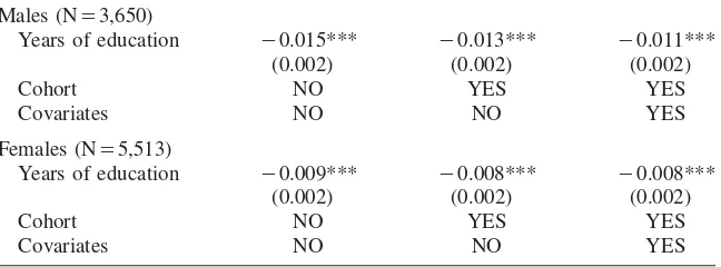
Table 1
Naı¨ve OLS estimates of the Probability of Death on Years of Education
Males (N⳱3,650)
Years of education ⳮ0.015*** ⳮ0.013*** ⳮ0.011***
(0.002) (0.002) (0.002)
Cohort NO YES YES
Covariates NO NO YES
Females (N⳱5,513)
Years of education ⳮ0.009*** ⳮ0.008*** ⳮ0.008***
(0.002) (0.002) (0.002)
Cohort NO YES YES
Covariates NO NO YES
Notes: Naı¨ve OLS estimates of the effect of years of education on the probability of dying between 1998 and 2005 of cohorts born between 1912 and 1922. Data are from the 1997–2005 POLS. Cohort refers to a quartic polynomial in cohort. Covariates include wave dummies, marital status, province, city size and ethnicity. Robust standard errors are given in parenthesis. *p-value⬍0.1, **p-value⬍0.05, ***p-value
⬍0.01
IV. Results
A. Naı¨ve OLS Estimates
Table 1 gives naı¨ve OLS estimates of the impact of an additional year of schooling on the probability of dying in the 1998–2005 period for cohorts born between 1912 and 1922. For males, the reduction in the probability of dying is 1.5 percentage points per additional year of schooling, and this falls to 1.1 points but still remains strongly significant when both a cohort trend (quartic polynomial) and covariates (marital status, ethnicity, province, and city size) are controlled for. For females, there is also a significant but slightly smaller effect of 0.8–0.9 percentage points. There is clearly a negative association between education and mortality in this popu-lation. Our aim is to establish whether the correlation has a causal element. First-stage Estimates
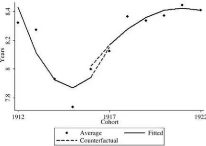
Figure 1a
Years of education by cohort. 1912–22 birth-year cohorts, males
Figure 1b
Years of education by cohort. 1912–22 birth-year cohorts, females
Data are from the 1997–2005 POLS. Fitted line is from a quadratic in cohort with the trend allowed to differ on either side of the reform threshold (as in the right-hand column of Table 2—lowest AIC value).
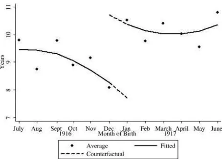
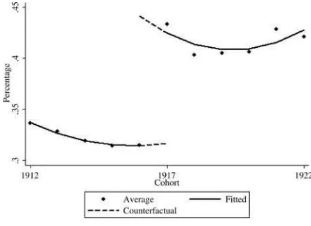
edu-Figure 2
Years of education by month-of-birth. Last six months of 1916 and first six months of 1917, males
cation was considered more necessary than for girls” (CBS 1931, p. 50). Given this, we do not pursue the estimation of a causal effect for women.
Figure 2, which shows, for males, years of schooling by month of birth for the last six months of 1916 and the first six months of 1917, confirms a discontinuity at January 1917, supporting the choice of this date for the reform threshold. Note that estimating the treatment effect using month-of-birth data is not feasible due to the small cell sizes at that level, particularly for the older cohorts. We do, however, check robustness in Section 4.5 to using six monthly and quarterly data.
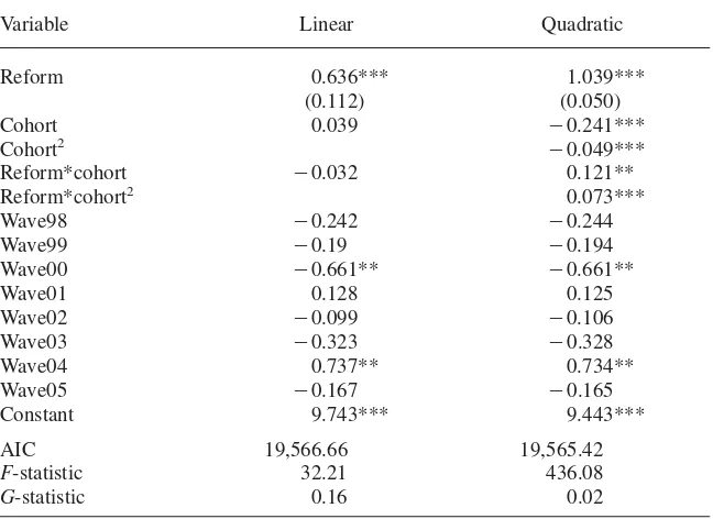
The first-stage OLS estimates presented in Table 2 indicate that the 1928 reform raised the average years of schooling of males by between seven months and one year depending on whether the cohort trends are specified as linear or quadratic. The reform indicator is strongly statistically significant in both models, which is confirmed by the extremely strong robustF-tests of the instrument, passing all cri-teria proposed in the literature (Bound, Jaeger, and Baker 1995; Staiger and Stock 1997; Stock and Yogo 2002).16TheG-tests indicate that both models are sufficiently
flexible and we have confirmed robustness to alternative specifications of the cohort trends, with the coefficient on the reform indicator always significant and lying in the range of 0.6–1.
Table 2
First-stage estimates of Years of Education on the Compulsory Schooling Law (N⳱3,650).
Variable Linear Quadratic
Reform 0.636*** 1.039***
(0.112) (0.050)
Cohort 0.039 ⳮ0.241***
Cohort2 ⳮ0.049***
Reform*cohort ⳮ0.032 0.121**
Reform*cohort2 0.073***
Wave98 ⳮ0.242 ⳮ0.244
Wave99 ⳮ0.19 ⳮ0.194
Wave00 ⳮ0.661** ⳮ0.661**
Wave01 0.128 0.125
Wave02 ⳮ0.099 ⳮ0.106
Wave03 ⳮ0.323 ⳮ0.328
Wave04 0.737** 0.734**
Wave05 ⳮ0.167 ⳮ0.165
Constant 9.743*** 9.443***
AIC 19,566.66 19,565.42
F-statistic 32.21 436.08
G-statistic 0.16 0.02
Notes: OLS estimates controlling for cohort trend and wave dummies. Estimations pertain to cohorts 1912– 22, for males. Data are from the 1997–2005 POLS. “Reform” is 1 if 1917 cohort or later. The “Cohort” variable is centered on the 1917 cohort. AIC is the Akaike Information Criterion.F-statistic is for test of significance of “reform,” and is robust to clustering at cohort level and heteroskedasticity.G-statistic is the test statistic of the flexibility of the cohort polynomial, which follows aF(J-K,N-J) distribution, whereJ
is the number of cohorts used in the estimation,Kis the number of parameters, andNis the number of observations (Lee and Card 2008). Standard errors (in parenthesis for “Reform”) are robust to heteroske-dasticity and clustering at the cohort level. *p-value⬍0.1, **p-value⬍0.05, ***p-value⬍0.01
C. Reduced Form Estimates
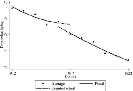
For male cohorts born between 1912 and 1922 present in the pooled POLS samples from 1997 to 2005, there is a small downward discontinuity at the 1917 threshold in the probability of dying before the end of 2005 (Figure 3). The respective reduced form estimate of the effect of the reform on mortality is negative in both models presented in Table 3, but the effect is not significant. Insignificance could simply be due to a lack of power, which is not a problem with the much larger RIO sample.
Figure 3
Proportion of the pooled 1997–2005 POLS sample that died before the end of 2005, by cohort
Fitted line is from a quadratic in cohort with the trend allowed to differ on either side of the reform threshold (as in the third column of Table 3—lowest AIC value). Cohorts 1912–1922, males.
corresponding graph produced from the POLS data (Figure 3).17Although the
dis-continuity at the reform threshold seems small, there is a small downward shift in the (linear) trend at that point. The corresponding reduced form estimates presented in the right-hand panel of Table 3 confirm that the 1928 reform induced changes that reduced the probability of dying before the age of 89 for individuals surviving to 81 by 2–3 percentage points, an effect that is strongly significant.
D. (Two Sample) Two Stage Least Squares Estimates
Irrespective of the specification, the 2SLS point estimate of the effect of years of education on mortality is negative and close to 0.03 in magnitude but is not signifi-cant (Table 4). The TS2SLS estimates, generated using the larger RIO sample, in-dicate that, for individuals surviving to age 81, an additional year of schooling significantly reduces the probability of dying before reaching 89 by just less than three percentage points.18Given that around 50 percent of males with six years of
schooling, corresponding to primary school completion, died between the ages of
17. Note that the average mortality rate in the 1998 RIO is higher than in the POLS data, which is due to the fact that the POLS data samples a new cross-section of survivors every year between 1998 and 2005.
Table 3
Reduced Form estimates of the Probability of Death on the Compulsory Schooling Law.
Variable Linear Quadratic Linear Quadratic
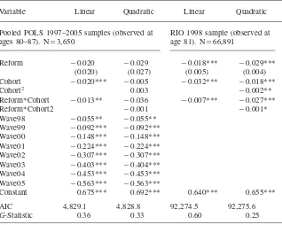
Pooled POLS 1997–2005 samples (observed at ages 80–87). N⳱3,650
RIO 1998 sample (observed at age 81). N⳱66,891
Reform ⳮ0.020 ⳮ0.029 ⳮ0.018*** ⳮ0.029***
(0.020) (0.027) (0.005) (0.004)
Cohort ⳮ0.020*** ⳮ0.005 ⳮ0.032*** ⳮ0.018***
Cohort2 0.003 ⳮ0.002**
Reform*Cohort ⳮ0.013** ⳮ0.036 ⳮ0.007*** ⳮ0.027***
Reform*Cohort2 ⳮ0.001 ⳮ0.001*
Wave98 ⳮ0.055** ⳮ0.055**
Wave99 ⳮ0.092*** ⳮ0.092***
Wave00 ⳮ0.148*** ⳮ0.148***
Wave01 ⳮ0.224*** ⳮ0.224***
Wave02 ⳮ0.307*** ⳮ0.307***
Wave03 ⳮ0.403*** ⳮ0.404***
Wave04 ⳮ0.453*** ⳮ0.453***
Wave05 ⳮ0.563*** ⳮ0.563***
Constant 0.675*** 0.692*** 0.640*** 0.655***
AIC 4,829.1 4,828.8 92,274.5 92,275.6
G-Statistic 0.36 0.33 0.60 0.25
Notes: Reduced Form OLS estimates of the impact of the 1928 Compulsory Schooling Law on the prob-ability of dying before the age of 89 for individuals surviving to at least 80. Estimations pertain to cohorts 1912–22, for males. “Reform” is 1 if 1917 cohort or later. AIC and G-test as in Table 2. Standard errors (in parenthesis for “Reform”) are robust to heteroskedasticity and clustering at the cohort level. *p-value
⬍0.1, **p-value⬍0.05, ***p-value⬍0.01
81 and 88, our estimates suggest that one extra year of schooling reduced the prob-ability of dying by 6 percent.
E. Robustness and Placebo Tests
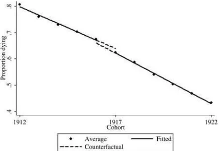
Figure 4
Eight-year mortality rate—proportion of the 1998 RIO sample that died before then end of 2005, by cohort
Fitted line is from a linear in cohort with the trend allowed to differ on either side of the reform threshold (as in the fourth column of Table 3—lowest AIC value). Cohorts 1912–22, males
Table 4
Regression Discontinuity estimates of the Probability of Death on Years of Education.
Variable Linear Quadratic
2SLS estimates from 1997–2005 POLS (observed at ages 80–87). (N⳱3,650)
Years of education ⳮ0.031 ⳮ0.028
(0.027) (0.025)
TS2SLS estimates from 1997–2005 POLS (N⳱3,650) and RIO 1998 followup (observed at age 81). (N⳱66,891)
Years of education ⳮ0.027*** ⳮ0.026***
(0.009) (0.004)
reliable cohort trend.19 The estimation is repeated using ten and three cohorts on
either side of the 1917 threshold (Table 5). Using ten cohorts brings the first-stage coefficient from the quadratic specification closer to that of the linear model, which increases somewhat.20 The reform indicator is still highly significant, with the
F-tests (not shown) showing no evidence of a weak instrument. Raising the bandwidth to ten cohorts increases the reduced form estimate somewhat for the linear model, yet decreases it for the quadratic specification. In both cases, the effect remains significant. As a result of the changes in the first-stage and the reduced form esti-mates, using a bandwidth of ten cohorts has little impact on the magnitude and significance of the TS2SLS estimate with the quadratic specification, but the estimate increases from 2.7 percentage points to 4.8 points, and remains highly significant, with the linear specification. Reducing the bandwidth to three cohorts has some impact on the first-stage and reduced form point estimates. These changes have very little impact on the TS2SLS estimate using the linear specification, but in the qua-dratic model an additional year of education is estimated to reduce the probability of death by only 1.2 points compared with an effect of 2.6 in the base case. The magnitude of the effect is therefore somewhat sensitive to the choice of bandwidth, with the range of estimates increasing to 1.2–4.8 points. But the effect remains strongly significant in all cases.
Our identification strategy relies on the assumption that all of the difference in mortality between the cohort immediately before the reform and the one immediately after the reform is attributable to the difference in education. This is more plausible when the time separating those two cohorts is less. Comparability between individ-uals born in the second half (last quarter) of 1916 and those born in the first half (first quarter) of 1917 should be greater than that between those born in all of 1916 and those born in 1917. However, in our case, using half-yearly or quarterly cohorts does not allow a more accurate definition of the threshold, and it increases variability since the cohort sizes get much smaller. For these reasons, we use birth-year cohorts in the base analysis and check robustness to higher frequency analysis. When doing so, we take account of possible season-of-birth effects (Doblhammer and Vaupel 2001; Doblhammer 2002) by including dummies for quarter-of-birth.
The first-stage estimates are very robust to replacing birth-year with half-year and quarter-of-birth cohorts (Table 5). As would be expected given the fall in cell sizes, significance of the reduced form estimates is reduced, but maintained at 5 percent in three out of four cases, while the point estimates change little. As a result, the TS2SLS point estimates are relatively robust, falling in magnitude from around a
19. Imbens and Kalyanaraman (2009) suggest a data dependent bandwidth choice rule, according to which the optimal bandwidth in the first stage is 4.31, which is very close to our chosen bandwidth of 5 and within the range of this and the smallest bandwidth used in the robustness analysis. Estimates using 4 cohorts on both sides of the threshold (not presented) are also extremely close to those obtained with 5 cohorts. The Imbens and Kalyanaraman rule indicates an optimal bandwidth of 1.6 in the reduced form but we have used 5 cohorts in the base case analysis since the same authors advise using the same bandwidth at both stages
The
Journal
of
Human
Resources
Table 5
Robustness to choice of bandwidth, frequency of running variable and use of 1998 POLS sample only in first-stage
First-Stage estimates Reduced Form estimates TS2SLS estimates
Linear Quadratic Linear Quadratic Linear Quadratic
Bandwidth
Base (five year) 0.636*** 1.039*** ⳮ0.018*** ⳮ0.029*** ⳮ0.027*** ⳮ0.026***
(0.112) (0.050) (0.005) (0.004) (0.009) (0.004)
Ten year 0.787*** 0.619*** ⳮ0.039*** ⳮ0.015** ⳮ0.048*** ⳮ0.024**
(0.075) (0.139) (0.006) (0.005) (0.009) (0.019)
Three year 0.819*** 1.197*** ⳮ0.021*** ⳮ0.015*** ⳮ0.023*** ⳮ0.012***
(0.058) (0.053) (0.002) (0.002) (0.003) (0.001)
Frequency of running variable
Base (year of birth) 0.636*** 1.039*** ⳮ0.018*** ⳮ0.029*** ⳮ0.027*** ⳮ0.026***
(0.112) (0.050) (0.005) (0.004) (0.009) (0.004)
Half year birth 0.671** 1.117** ⳮ0.019** ⳮ0.027** ⳮ0.023* ⳮ0.022**
(0.308) (0.412) (0.008) (0.010) (0.013) (0.010)
Quarter of birth 0.672** 1.062** ⳮ0.015** ⳮ0.019* ⳮ0.022 ⳮ0.018
(0.307) (0.467) (0.006) (0.010) (0.013) (0.012)
Only 1998 POLS used in first stage
First stage (Reform) 0.760** 0.917* — — ⳮ0.023** ⳮ0.031**
(0.297) (0.421) (0.011) (0.015)
three percentage point reduction in the probability of death with an extra year of schooling to a two point reduction. When quarter-of-birth cohorts are used, and so the cell sizes become very small, significance rises just above the 10 percent thresh-old (p⳱0.103 for the linear model, andp⳱0.133 for the quadratic).
TS2SLS is consistent under the assumption that the two samples are drawn from the same underlying population (Angrist and Krueger 1992; Arellano and Meghir 1992). This is not strictly true in our case since the first stage is estimated using the pooled POLS cross-section samples of the 1997–2005 populations, while the second stage is estimated using the RIO one-third sample of the 1998 population followed to 2005.21Consistency of the TS2SLS estimator would be threatened if the impact
of the reform on the education of the 1998 population differed from its effect in the other populations from which samples are drawn for the first stage. A test of the joint significance of a full set of reform-wave interactions in the first stage with 1998 as the reference rejects the null in both specifications, suggesting that the effect does indeed vary. Yet, individually, only the effect in the 1999 sample is significantly different from that in the 1998 sample, and only at the 10 percent level. Moreover, using only the 1998 POLS to estimate the first-stage changes the point estimates of the reform effect relatively little (Table 5). The standard errors increase greatly, which is to be expected given the sample size falls from 3,650 to 833, but signifi-cance is maintained at 10 percent or less. The TS2SLS estimates are robust to using 1998 data only in the first stage. The point estimates are in the range of 2.3–3.1 points and are significant at 5 percent.
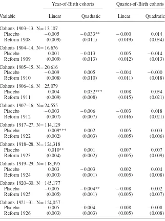
While the statistical power provided by the RIO sample size is clearly an advan-tage, one might worry that this is responsible for detecting an effect that is apparent but not real. To investigate this we test ten placebo reforms—five on each side of the actual reform. Keeping pre and post actual reform samples separate and using a five-year bandwidth to ensure comparability with our base scenario (Imbens 2004; Imbens and Lemieux 2008), we place artificial thresholds at each cohort from 1908 to 1912, and at each cohort from 1922 to 1926. Five of the 20 tests conducted across the two reported specifications reject the null of no effect of the placebo reform (Table 6, Columns 1 and 2), which is obviously in excess of the one rejection at the 5 percent level of significance that would be expected to occur by chance. However, significance of a placebo only ever occurs with one of the two specifications and the point estimate from the other specification typically differs greatly. For no pla-cebo reform is there any indication of the strongly significant and consistently es-timated effects of the 1928 reform observed in the bottom half of Table 3. Signifi-cance of the fictitious reforms could be due to fluctuations caused, for example, by the business cycle. This is unlikely for the highest possible frequency for our running variable—quarter-of-birth. None of the 20 placebo tests performed at this frequency rejects the null (Table 6, Columns 3 and 4), in contrast to the actual reform which is consistently estimated and statistically significant when treatment is defined by quarter of birth (Table 5). This gives us confidence that the significant effects are
Table 6
Placebo tests—Reduced Form estimates of the Probability of Death on Fictitious Reforms.
Year-of-Birth cohorts Quarter-of-Birth cohorts
Variable Linear Quadratic Linear Quadratic
Cohorts 1903–13. N⳱13,107
Placebo ⳮ0.005 ⳮ0.033** ⳮ0.000 0.014
Reform 1908 (0.009) (0.011) (0.019) (0.034)
Cohorts 1904–14. N⳱16,676
Placebo 0.001 ⳮ0.013 0.005 ⳮ0.014
Reform 1909 (0.009) (0.013) (0.012) (0.013)
Cohorts 1905–15. N⳱20,616
Placebo ⳮ0.009 0.005 ⳮ0.004 ⳮ0.000
Reform 1910 (0.008) (0.010) (0.011) (0.018)
Cohorts 1906–16. N⳱25,079
Placebo 0.004 0.032*** 0.008 0.034
Reform 1911 (0.009) (0.008) (0.015) (0.021)
Cohorts 1907–16. N⳱24,555
Placebo ⳮ0.003 ⳮ0.006 ⳮ0.003 0.018
Reform 1912 (0.007) (0.007) (0.016) (0.021)
Cohorts 1917–27. N⳱114,129
Placebo 0.009*** 0.002 0.005 0.003
Reform 1922 (0.002) (0.003) (0.005) (0.006)
Cohorts 1918–28. N⳱124,318
Placebo 0.010** 0.001 0.007 0.007
Reform 1923 (0.004) (0.002) (0.005) (0.009)
Cohorts 1919–29. N⳱118,395
Placebo 0.003 ⳮ0.003 0.002 0.004
Reform 1924 (0.003) (0.001) (0.005) (0.008)
Cohorts 1920–30. N⳱145,177
Placebo ⳮ0.005 ⳮ0.004** ⳮ0.008 0.002
Reform 1925 (0.005) (0.001) (0.005) (0.007)
Cohorts 1921–31. N⳱154,057
Placebo ⳮ0.005 ⳮ0.004 ⳮ0.008 ⳮ0.008
Reform 1926 (0.003) (0.003) (0.005) (0.008)
Notes: OLS estimates on RIO 1998 data with mortality followup, for males. “Placebo Reform” refers to the artificial reform at the birth-year cohort indicated. Columns 1 and 2 are based on yearly cohorts; Columns 3 and 4 are based on quarter-of-birth cohorts. Robust standard errors in parenthesis. *p-value
not simply attributable to the large sample size, but rather reflect a real effect of education expansion at the threshold.
V. Discussion
A compulsory schooling law introduced in the Netherlands in 1928 increased the schooling of Dutch males by 0.6–1.0 years, on average. Using this as a strong and exogenous instrument for educational attainment, along with directly observed mortality data on a random one-third of the population, we find that edu-cation significantly reduces mortality in old age. For a Dutch male surviving to the age of 81, an additional year of schooling reduces the probability that he will die before reaching 89 by slightly less than three percentage points relative to a baseline probability of 50 percent. This suggests that the well-documented large correlation between education and health outcomes is not spurious but stems (at least partly) from a causal effect of education on health, and consequently longevity.
This conclusion is consistent with that of Lleras-Muney (2005), who finds that increased schooling resulting from education reforms introduced in the United States between 1915 and 1939 reduced mortality significantly. Although the different ages of the samples impedes comparability, our estimate of an extra year of schooling reducing the probability of death over an eight-year period from the age of 81 by slightly less than 6 percent is perhaps more plausible than Lleras-Muney’s (2005; 2006) tenfold larger IV estimate of about 60 percent for cohorts aged 35–69. The magnitude and significance of the latter estimate have been found not robust to controlling for state specific cohort trends that may capture the effects of mortality-reducing public health measures coincident with compulsory schooling laws (Ma-zumder 2008). Our estimate is identified from a discrete and marked jump in school-ing due to a nationally implemented reform that is less likely to have coincided with some other factor responsible for shifting mortality from its trend over the ten-year period examined.
Figure 5
Proportion finishing high school by cohort. Data are from the 1997–2005 POLS
Fitted line is from a quadratic in cohort with the trend allowed to differ on either side of the reform threshold. Cohorts 1912–22, males
our study of individuals between the ages of 81 and 89 facing a mortality rate of 50 percent.
The British reforms examined by Clark and Royer raised the minimum age at which a child was permitted to leave secondary school from 14 to 15 in 1947 and from 15 to 16 in 1972. These corresponded to increases in the number of years of compulsory schooling to 10 and 11 respectively. The 1928 Dutch reform exploited in the present paper took effect at a much lower base level of education, raising the compulsory years of schooling from six to seven. Diminishing health returns to education may partly account for the different findings of the two studies. A priori diminishing returns is a plausible hypothesis—one might expect large health returns to basic reading and writing skills that should be most crucial to the processing of health related information. Lleras-Muney (2005) finds evidence of a convex rela-tionship between mortality and education instrumented by compulsory schooling laws.22Auld and Sidhu (2005) show that the association between health, measured by work limitations, and schooling in the United States diminishes beyond high school level and find evidence of a causal effect only before high school graduation. Returns to the 1928 Dutch reform may be particularly high not only because it compelled an extra year of schooling at a relatively low level but because it induced a change in the nature of the education experienced. Since primary school in the Netherlands consists of 6 years, the reform required entry to secondary school. Fig-ure 5 shows that the rate of secondary school completion increased by more than
ten percentage points for the first cohort affected by the reform. It would appear that the reform was successful not only in forcing children to start secondary school but also induced many to complete this level. Secondary schooling exposed children to a new curriculum and a different group of peers. In contrast, the British education reforms studied by Clark and Royer extended the length of compulsory secondary schooling and, to some extent, can be characterized as entailing more of the same. The 1947 reform involved no change of curriculum and, given that it affected 50 percent of the cohort, did not result in large changes in peer group exposure. Al-though monetary returns to this reform have been clearly demonstrated (Oreopoulos 2006; Clark and Royer 2010), it could well be that its nature precluded the generation of substantial health returns.
Given that year-of-birth is a relatively coarse running variable in an RDD, one might worry that other events occurred around the threshold that may have had long-run consequences for the health and mortality of cohorts born at that time. The robustness of our estimates to using half-year and quarter-of-birth cohorts makes it less likely that factors other than the 1928 education reform are responsible for the decline in mortality. Nonetheless, it is worth considering whether there are plausible alternative explanations. The 1917 cohort was born during World War I. Despite being neutral in the war, the Netherlands was affected by it—most notably through the reduced supply of food (Abbenhuis 2006, pp. 187–194). But the war lasted from 1914 to 1918 and there seems little reason to expect its long-run health consequences to differ much between those born in 1916 and those born in 1917.
Using a unique historical data set, Van den Berg, Lindeboom, and Portrait (2006) find that individuals born during a recession in the Netherlands in the 19th century faced higher mortality risks than those born during an economic boom. The effect is largest between the ages of 15 and 34 but it remains significant even up to the age of 90. Although our data covered a later period, this study suggests that one should check for abrupt changes in macroeconomic conditions around the threshold. The Dutch economy grew rapidly 1914–16, stagnated 1916–17 and grew even more rapidly between 1918 and 1920.23 According to the estimates of Van den Berg,
Lindeboom, and Portrait, the recession between 1916 and 1917 should have raised mortality around the threshold. The discrete fall observed in mortality at this point, evident even in quarter-of-birth comparisons, does not therefore appear attributable to changing macroeconomic conditions. Another major health event in this period was the 1918 “Spanish Flu” Pandemic. Almond (2006) finds that, in the United States, individuals who were in utero at the time of the pandemic experienced higher rates of physical disability, as well as lower socioeconomic status, in their middle age. In the Netherlands, the pandemic struck in the autumn of 1918, almost two years after our January 1917 threshold. If there are long-run consequences for health, then this would tend to raise mortality in our post-reform cohorts. This is inconsistent with what we observe and so not a plausible alternative explanation of our results.
Figure 6
Eight-year mortality rate-proportion of the 1998 RIO sample that died in the period 1998–2005, by cohort
Fitted line is from a linear in cohort with the trend allowed to differ on either side of the reform threshold. Cohorts 1912–22, females.
Because these and other events might be expected to impact equally on women and men, examination of the trend in female mortality over the relevant cohorts can be used to gauge whether extraneous events provide a plausible explanation for the observed decline in male mortality at the threshold. As can be seen in Figure 6, there is no discontinuity in female mortality at the 1917 cohort (the reduced form point estimate isⳮ0.001 with standard error of 0.003). Given that we also find no significant impact of the reform on the schooling of females, this further increases the likelihood that the observed fall in mortality among men is due to their increased educational attainment, rather than some coincidental other factor.
Our IV estimates of the impact of schooling on mortality are larger than those obtained assuming schooling to be exogenous.24Instrumenting is frequently found
to raise the estimated impact of education on earnings (for example, Card 1999) and this has also been observed in estimates of the health returns to education (Arkes 2003; Arendt 2005; Lleras-Muney 2005; Oreopoulos 2006; Silles 2009). Measure-ment error is a possible explanation but heterogeneity in the returns to education is a more convincing one. RDD IV identifies the LATE among compliers at the thresh-old of the 1928 reform (Hahn, Todd, and Van der Klaauw 2001; Van der Klaauw 2002; Imbens and Lemieux 2008), which may differ considerably from the average treatment effect on the treated (ATET) that OLS seeks to estimate. This interpretation implies that health returns are highest among those who would not have stayed on
at school had the minimum years of schooling not been increased. This is not par-adoxical once it is recognized that, relative to monetary returns, health returns are unlikely to play an important role in the decision to stay on at school. Further, particularly in the 1920s, individuals facing the greatest credit constraints may well have had higher than average potential returns—both monetary and nonmonetary— to education. Diminishing returns to education also may contribute to the discrepancy between the naı¨ve OLS and IV estimates. Using parental education as instruments, which mainly induce changes in post-high school education, Auld and Sidhu (2005) find IV estimates of health returns smaller than naı¨ve OLS estimates. This contrasts with what is found when compulsory schooling laws are used as instruments, which provides variation around a lower level of education (Arendt 2005; Lleras-Muney 2005; Oreopoulos 2006; Silles 2009).
Two broad hypotheses have been advanced to explain an impact of education on health. According to the first, education raises the productivity of investments in health, including medical care, through information acquisition and processing skills (Grossman 1972). This is perhaps less relevant in the context of universal health insurance and limited inequality in access to medical care in the Netherlands (Van Doorslaer, Masseria, and Koolman 2006). The second hypothesis is that education operates through health behavior (Muurinen 1982). Empirical studies confirm that the lower educated indulge in less healthy behavior (Feinstein et al. 2006; Cutler and Lleras-Muney 2008) and that lifestyle acts as a mediator between education and health (Contoyannis and Jones 2004; Balia and Jones 2008). The cohorts studied in this paper were 42–52 when the U.S. Surgeon General’s Report on Smoking and Health was published in 1964. U.S. studies report that the better educated were more likely to quit smoking, or not take it up, after the publication of evidence on its risks (De Walque 2007; Grimard and Parent 2007). Although most smoking-related deaths occur before the age of 80, Peto et al. (1992) estimate that 39 percent of deaths of Dutch males in 1995 above the age of 70 were smoking-related. We investigated whether there was any evidence of a mechanism through smoking be-havior by comparing the estimated treatment effects of education on different causes of death. While we did find a significant effect on deaths from respiratory diseases and on all deaths categorized as smoking attributable mortality (U.S. Department of Health and Social Service 1989; Peto et al. 1992), there was no consistent evidence of a larger effect on these than on other causes of death (results available upon request).
A distinguishing feature of our study is that we estimate the impact of schooling on mortality for individuals aged above 81. This allows us to test whether there are very long-run nonmonetary returns to education but it also means that we miss any impact that education may have on the probability of survival to old age. If education raises this probability, then our estimate of a 6 percent reduction in the eight-year mortality rate will understate the impact of education on mortality in old age since low-educated survivors, having overcome their education-related disadvantage, will have an advantage over their highly education comparators in health determinants that are not related to education. So, the long-run health returns to education may be even greater than we estimate.
estimated longevity returns may be more indicative of those to be expected from education policies being enacted, or considered, in the developing world today than they are of returns to rich world policies. That said, our estimates suggest that evolution of longevity of the elderly populations in developed countries, which is of fundamental importance to the design of pension and health policy, will depend on education experiences in early life many decades ago.
References
Abbenhuis, Maartje. 2006. “The Art of Staying Neutral: The Netherlands in the First World War, 1914–1918.” Amsterdam University Press, http://dare.uva.nl/aup/en/record/216555. Akaike, Hirotugu. 1974. “A New Look at the Statistical Model Identification.”IEEE
Transactions on Automatic Control19(6):716–23.
Albouy, Valerie, and Laurent Lequien. 2009. “Does Compulsory Education Lower Mortality?”Journal of Health Economics28(1):155–68.
Almond, Douglas. 2006. “Is the 1918 Influenza Pandemic Over? Long-term Effects of in Utero Influenza Exposure in the Post-1940 U.S. Population.”Journal of Political Economy114(4):672–712.
Angrist, Joshua D., and Alan B. Krueger, 1992. “The Effect of Age at School Entry on Educational Attainment: An Application of Instrumental Variables with Moments from Two Samples.”Journal of the American Statistical Association87(418):328–36. Angrist, Joshua D, and Jorn-Steffen Pischke. 2009. Mostly Harmless Econometrics.
Princeton: Princeton University Press.
Arellano, Manuel, and Costas Meghir. 1992. “Female Labour Supply and On-the-Job Search: An Empirical Model Estimated Using Complementary Data Sets.”Review of Economic Studies59(3):537–59.
Arendt Jacob N. 2005. “Does Education Cause Better Health? A Panel Data Analysis Using School Reforms for Identification.”Economics of Education Review24(2):149–60. Arendt Jacob N. 2008. “In Sickness and in Health till Education Do Us Part: Education
Effects on Hospitalization.”Economics of Education Review27(2):161–72.
Arkes, Jeffrey. 2003. “Does Schooling Improve Health?” Working paper DRU-3051, RAND Corporation, Santa Monica.
Auld, M. Christopher, and Nirmal Sidhu. 2005. “Schooling, Cognitive Ability, and Health.”
Health Economics14(10):1019–34.
Bago d’Uva, Teresa, Owen O’Donnell, and Eddy van Doorslaer, 2008. “Differential Health Reporting by Education Level and its Impact on the Measurement of Health Inequalities among Older Europeans.”International Journal of Epidemiology37(6):1375–83. Balia, Silvia, and Andrew M. Jones. 2008. “Mortality, Lifestyle and Socio-Economic
Status.”Journal of Health Economics27(1):1–26.
Baum, Christopher F., Mark E. Schaffer, and Steven Stillman. 2007. “Enhanced Routines for Instrumental Variables/GMM Estimation and Testing.” Boston College Economics Working Paper no. 667.
Behrman, Jere R., and Mark R. Rosenzweig. 2004. “Returns to Birthweight.”The Review of Economics and Statistics86(2):586–601.
Berger, Mark C., and J. Paul Leigh. 1989. “Schooling, Self-Selection, and Health.”The Journal of Human Resources24(3):433–55.
Bound, John, David A. Jaeger, and Regina M. Baker. 1995. “Problems with Instrumental Variables Estimation when the Correlation Between the Instruments and the Endogenous Explanatory Variables is Weak.”Journal of the American Statistical Association
90(430):443–50.
Card, David E. 1999. “The Causal Effect of Education on Earnings.” inThe Handbook of Labor Economics, Volume 3A, ed. Orley Ashenfelter and David E. Card, 1801–64. Amsterdam: Elsevier.
Case Anne, Angela Fertig, and Christina Paxson. 2005. “The Lasting Impact of Childhood Health and Circumstance.”Journal of Health Economics24(2):365–89.
Centraal Bureau voor de Statistiek (CBS). 1931. Statistiek van het Gewoon en Uitgebreid Lager Onderwijs. Centraal Bureau voor de Statistiek. ’s-Gravenhage : Algemeene Landsdrukkerij.
Centraal Bureau voor de Statistiek (CBS). 2008. “Hoogopgeleiden Leven Lang en Gezond” in:Gezondheid en zorg in cijfers, ed. Van Hilten, O., and A.M.H.M. Mares. CBS, The Hague, the Netherlands.
Clark, Damon, and Heather Royer. 2010. “The Effect of Education on Adult Health and Mortality: Evidence from Britain.” NBER Working Paper series 16013. May 2010. Contoyannis, Paul, and Andrew M. Jones. 2004. “Socio-Economic Status, Health and
Lifestyle.”Journal of Health Economics23(5):965–95.
Cutler, David M., and Adriana Lleras-Muney. 2008. “Education and Health: Evaluating Theories and Evidence.” inMaking Americans Healthier: Social and Economic Policy As Health Policy,ed. Robert F. Schoeni, James S. House, George A. Kaplan and H. Pollack. National Poverty Center Series on Poverty and Public Policy.
De Graaf, Jacoba H. 2000. “Leerplicht en Recht op Onderwijs.”Ars Aequi Libri,University of Amsterdam Dissertation series.
Deary, Ian. 2008. “Why do Intelligent People Live Longer?”Nature456:175–76. Devereux, Paul J., and Robert A. Hart. 2010. “Forced to be Rich? Returns to Compulsory
Schooling in Britain.”Economic Journal120(549):1345–64.
De Walque, Damien. 2007. “Does Education Affect Smoking Behaviors? Evidence Using the Vietnam Draft as an Instrument for College Education.”Journal of Health Economics
26(5):877–95.
Doblhammer, Gabriele, and James W. Vaupel. 2001. “Lifespan Depends on Month of Birth.”Proceedings of the National Academy of Sciences of the United States of America
98(5):2934–39.
Doblhammer, Gabriele. 2002. “Differences in Lifespan by Month of Birth for the United States: The Impact of Early Life Events and Conditions on Late Life Mortality.” Max Planck Institute for Demographic Research Working Paper 2002–19.
Dodde, Nan. 2000. “Een Geschiedenis van de Leerplicht.” In:Recht doen aan zorg. 100 jaar Leerplicht in Nederland.ed. Ton van der Hulst, and Dolf van Veen. Leuven/ Apeldoorn.
Feinstein, Leon, Ricardo Sabates, Tashweka M. Anderson, Annik Sorhaindo, and Cathie Hammond. 2006. “The Effects of Education on Health: Concepts, evidence and policy implications”Paris: Organisation for Economic Co-operation and Development (OECD). Fuchs, Viktor R. 1982. “Time Preference and Health: An Exploratory Study.” InEconomic
Aspects of Health,ed. V. Fuchs. Chicago: The University of Chicago Press. Gielen, Wilhelmus J.G.M. 1984. Het Wondere Ambt: het Rijksschooltoezicht en de
Toepassing van de Lager-Onderwijswet 1920 Gedurende de Jaren 1921 tot en met 1930. Doctoral Dissertation, University of Nijmegen, the Netherlands.
Grimard, Franque, and Daniel Parent. 2007. “Education and Smoking: Were Vietnam War Draft Avoiders Also More Likely to Avoid Smoking?”Journal of Health Economics
Grossman, Michael. 1972. “On the Concept of Health Capital and the Demand for Health.”
Journal of Political Economy80(2):223–55.
Grossman, Michael, and Robert Kaestner 1997. “Effects of Education on Health.” inThe Social Benefits of Education,ed. J. R. Berhman and N. Stacey. Ann Arbor: University of Michigan Press.
Hahn, Jinyong, Petra Todd, and Wilbert Van der Klaauw. 2001. “Identification and Estimation of Treatment Effects with a Regression-Discontinuity Design.”Econometrica
69(1):201–209.
Hentzen, Cassanius. 1928. “De Financieele Gelijkstelling 1920–1925” In: Politieke Geschiedenis Lager Onderwijs in Nederland, R.K. Centraal Bureau voor Onderwijs en Opvoeding, ’s-Gravenhage, the Netherlands.
Hentzen, Cassanius. 1932. “De Financieele Gelijkstelling 1926–1929.” In: Politieke Geschiedenis Lager Onderwijs in Nederland, R.K. Centraal Bureau voor Onderwijs en Opvoeding, ’s-Gravenhage, the Netherlands.
HSG, 1946/1947. Handelingen der Staten-Generaal. Bijlagen 1946–1947. 459.3: p.4. HTK, 1946/1947. Handelingen Tweede Kamer 1946–1947. 459: p. 1968
Idenburg, Philip J. 1964. Schets van het Nederlandse Schoolwezen. Groningen: Wolters. Imbens, Guido W. 2004. “Nonparametric Estimation of Average Treatment Effects Under
Exogeneity: A Review.”The Review of Economics and Statistics86(1):4–29. Imbens, Guido W., and Thomas Lemieux. 2008. “Regression Discontinuity Designs: A
Guide to Practice.”Journal of Econometrics142(2):615–35.
Imbens, Guido W., and Karthik Kalyanaraman. 2009. “Optimal Bandwidth Choice for the Regression Discontinuity Estimator.” NBER Working Paper 14726.
Inoue, Atsushi, and Gary Solon. 2010. “Two-Sample Instrumental Variables Estimators.The Review of Economics and Statistics92(3):557–61.
Lee, David S., and David Card. 2008. “Regression Discontinuity Inference with Specification Error.”Journal of Econometrics142(2):655–74.
Lee, David S., and Thomas Lemieux. 2010. “Regression Discontinuity Designs in Economics.”Journal of Economic Literature48(2):281–355.
Lleras-Muney, Adriana. 2005. “The Relationship Between Education and Adult Mortality in the United States.”Review of Economic Studies72(1):189–221.
———. 2006. “Erratum: The Relationship Between Education and Adult Mortality in the United States.”Review of Economic Studies73(3): 847.
Mackenbach, Johan P., Irina Stirbu, Albert-Jan R. Roskam, Maartje M. Schaap, Gwenn Menvielle, Mall Leinsalu, and Anton E. Kunst. 2008. “Socioeconomic Inequalities in Health in 22 European Countries.”New England Journal of Medicine358(23):2468–81. Mandemakers, Cornelis A. 1996.Gymnasiaal en Middelbaar Onderwijs: Ontwikkeling,
Structuur, Sociale Achtergrond en Schoolprestaties, Nederland, ca. 1800–1968. Doctoral dissertation, Erasmus University Rotterdam.
Mazumder, Bhaskar. 2008. “Does Education Improve Health? A Reexamination of the Evidence from Compulsory Schooling Laws.”Federal Reserve Bank of Chicago Economic Perspectives33(2):2–16.
Meijsen, Justus H. 1976.“Lager onderwijs in de spiegel der geschiedenis.”’s Gravenhage, the Netherlands
Muurinen, Jaana-Marja. 1982. “Demand for Health: A Generalised Grossman Model.”
Journal of Health Economics1(1):5–28.
Oreopoulos, Philip. 2006. “Estimating Average and Local Average Treatment Effects of Education when Compulsory School Laws Really Matter.”American Economic Review
96(1):152–75.
Peto, Richard, Alan D. Lopez, Jillian Boreham, Michael Thun, and Clark Heath. 1992. “Mortality from Tobacco in Developed Countries: Indirect Estimation from National Vital Statistics.”Lancet339:1268–78.
SHARE, 2007. “Documentation of Generated Variables in SHARE release 2.0.1” Retrieved from http://www.share-project.org/t3/share/index.php?id⳱74.
Silles, Mary A. 2009. “The Causal Effect of Education on Health: Evidence from the United Kingdom.”Economics of Education Review28(1):122–28.
Smith, James P., and Richard Kington. 1997. “Demographic and Economic Correlates of Health in Old Age.”Demography34(1):159–70.
Spasojevic, Jasmina. 2003. ”Effects of Education on Adult Health in Sweden: Results from a Natural Experiment.” PhD Dissertation. New York: City University of New York Graduate Center.
Staatsblad 1929, number 335. Official Bulletin of the State.
Staiger, Douglas, and James H. Stock. 1997. “Instrumental Variables Regression with Weak Instruments.”Econometrica65(3):557–86.
Sterringa, Gerben. 1934. Leerplicht en Leerplichtwet, J.B. Wolters Uitgevers-Maatschappij, Groningen, The Netherlands.
Stock, James H., and Motohiro Yogo. 2002. “Testing for Weak Instruments in Linear IV Regression.” NBER Technical Working Paper 284 (Revised 2004).
Thistlethwaite, Donald, and Donald Campbell. 1960. “Regression-Discontinuity Analysis: An Alternative to the Ex Post Facto Experiment.”Journal of Educational Psychology51: 309–17.
Trochim, William M.K. 1984.Research Design for Program Evaluation: the Regression-Discontinuity Approach.Beverly Hills, Calif.
U.S. Department of Health and Human Services. 1989. “Reducing the Health Consequences of Smoking: 25 Years of Progress.” A Report of the Surgeon General, Rockville, Maryland: Public Health Service, Centers for Disease Control, Office on Smoking and Health, 1989, (DHHS Publication No (CDC) 89-8411.).
Van den Berg, Gerard, Maarten Lindeboom, and France Portrait. 2006. “Economic Conditions Early in Life and Individual Mortality.”American Economic Review
96(1):290–302.
Van der Klaauw, Wilbert. 2002. “Estimating the Effect of Financial Aid Offers on College Enrollment: a Regression Discontinuity Approach.”International Economic Review
43(4):1249–87.
———. 2008. “Regression–Discontinuity Analysis: A Survey of Recent Developments in Economics.”Labour22(2):219–45.