Treatment Close to the Average?
Evidence from Fertility and Labor Supply
Avraham Ebenstein
a b s t r a c t
The local average treatment effect (LATE) may differ from the average treatment effect (ATE) when those influenced by the instrument are not representative of the overall population. Heterogeneity in treatment effects may imply that parameter estimates from 2SLS are uninformative regarding the average treatment effect, motivating a search for instruments that affect a larger share of the population. In this paper, I present and estimate a model of home production with heterogeneous costs and benefits to fertility. The results indicate that a sex-preference instrument in Taiwan produces IV estimates closer to the estimated ATE than in the United States, where sex preference is weaker.
I. Introduction
One of the most important and studied social trends of the 20th century is the dramatic decline in fertility rates among industrialized nations, and a concurrent rise in the labor supply of married women (Goldin 1995). Identifying the causal link between fertility and female labor force participation is difficult, however, since it may be that the decision to work and the decision to have another child are jointly de-termined (Willis 1973). Understanding this connection is of interest to social scientists trying to understand intrahousehold allocations, but now also has immediate policy
Avraham Ebenstein is a Robert Wood Johnson Scholar in Health Policy at Harvard University. The author thanks David Card, Ronald Lee, seminar participants at the UC-Berkeley Labor Lunch and Academia Sinica (Taipei, Taiwan), and three anonymous referees for helpful comments. Special thanks to Ethan Jennings and Sanny Liao for translation of all Taiwan survey documentation. The author would also like to acknowledge helpful guidance from Alberto Abadie, Jerome Adda, David Albouy, Rodney Andrews, Josh Angrist, Richard Crump, Tatyana Deryugina, Simon Galed, Gopi Shah Goda, Jonathan Gruber, Jane Leber Herr, Guido Imbens, Radha Iyengar, Damon Jones, Marit Rehavi, Claudia Sitgraves, Kevin Stange, An-Chi Tung, and Robert Willis. The data used in this article can be obtained beginning May 2010 through April 2013 from Avraham Ebenstein, Harvard University, 1730 CGIS S408, Cambridge, MA 02138, aebenste@rwj.harvard.edu.
½Submitted July 2007; accepted May 2008
ISSN 022-166X E-ISSN 1548-8004Ó2009 by the Board of Regents of the University of Wisconsin System
relevance. Many developed countries, including Taiwan,1are currently engaged in ini-tiatives to encourage fertility (Chamie 2004). Appropriate policy design is dependent on an understanding of the financial incentives already embedded in fertility decisions, including the cost in foregone wages to the mother of an additional child.
In order to identify the causal link between fertility and female labor supply, researchers have focused on instrumental variables (IV) that exploit exogenous sour-ces of variation in family size. Bronars and Grogger (1994) find that among mothers who are forced by a twin birth to have an additional child, the estimated impact is only significant for mothers having out-of-wedlock births. In a paper that motivated this project, Angrist and Evans (1998) find that the Ordinary Least Squares (OLS) estimator overstates the causal impact of fertility on labor supply when fertility is induced by the preference among couples to have at least one child of each sex. In both analyses, the authors conclude that higher fertilityper sehas a smaller impact on the labor supply of mothers than what is implied by the simple correlation be-tween fertility and labor supply. In light of the widespread and persistent use of sex composition as an instrument for fertility (Cruces and Galiani 2007, Conley and Glauber 2006), the generalizability of these estimated treatment effects is a con-cern.
The existing IV estimates are subject to two primary limitations. The first limita-tion is that instruments which are only weakly correlated with the regressor of inter-est may yield unstable parameter inter-estimates (Bound et al. 1995). The second limitation is that IV will only consistently estimate the treatment effect for those influenced by the instrument (Imbens and Angrist 1994). If treatment effects are het-erogenous in the population, this may not be informative regarding how theaverage
mother’s labor supply is affected by her number of children (Angrist 2004; Heckman and Vytlacil 2000). These concerns have motivated the search for instruments that affect larger and possibly more representative subpopulations (Oreopoulos 2006).
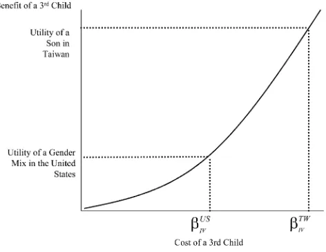
Taiwan, a highly industrialized country with widespread son preference, is an al-most ideal setting in which to examine the causal link between fertility and female labor supply. Mothers in Taiwan have similar labor force participation rates to their American counterparts, but are more likely to be swayed by sex preferences.2In the context of fertility and labor supply, it may be that an instrument based on sex pref-erence induces mothers with lower than average costs to childbearing to have an ad-ditional child. In this setting, IV, which estimates the treatment effect among those affected by the instrument, will generally estimate the average effect over subsam-ples of individuals with increasingly greater costs to an additional child as the inten-sity of the instrument increases (Figure 1).
I present a model of home production in which parents have preferences over the number and sex of their children, and heterogeneity is allowed in the benefits and costs to childbearing. Using census data from Taiwan and the United States, I esti-mate the model which indicates that the average treatment effect of a third child on a mother’s probability of working is -12.6 percent in Taiwan and -12.6 percent in the United States for mothers 21 to 35 years of age. The results imply that the IV estimate for the United States (-9.7 percent) may be estimated on a group of
1. http://www.taipeitimes.com/News/taiwan/archives/2007/08/25/2003375752 2. Author’s calculations, shown in Table 1.
mothers who experience lower than average costs to childbearing, whereas for Tai-wan the IV estimate (-12.4 percent) is closer to the model estimate. The results sug-gest that applied econometricians should interpret IV estimates with caution when treatment effects are heterogeneous and agents observe their private cost (or benefit) of the behavior in question, since stronger instruments will induce individuals with higher costs (or benefits) of treatment to comply with the instrument. The lesson for policymakers is that inducing fertility may be more difficult than anticipated, in light of the large cost in foregone earnings associated with having a third child.
The remainder of the paper is laid out as follows. In Section II, I present a theo-retical model of a mother’s joint determination of fertility and labor supply, and out-line the econometric strategy used to estimate the model. In Section III, I present the empirical results of OLS, IV, and structural estimation of the labor supply models. Section IV concludes the paper.
II. Causal Modeling of Fertility and
Labor Supply
A. Theoretical Model
Suppose that mothers spend a proportion of timehengaged in market activity and 12hengaged in home production. Let brepresent the time cost of an additional Figure 1
Causal Effects Estimated by Instrumental Variables and the Strength of the Instru-ment
child, and letacapture factors that affect hours worked unrelated to a mother’s num-ber of children. Suppose also that mothers vary in the time cost of childbearing and in their taste for home production such thatbandamay differ between mothers. The model is focused on the impact of a mother’s third childK3on her labor supply. The
causal relationship between fertility and motheri’s labor supply derived from the the-oretical model is given by the following equation3:
hi¼12ai2biK3i
ð1Þ
Let the value of a child of any sex be given bygiand the premium to having at
least one son be given byui. The decision to have a third child K3i is determined
by mothers comparing the value of a child in terms ofgianduito the foregone wages
associated with having that childwbi, where the wagewis assumed constant across
mothers for simplicity.4Consider an instrumentZ, which is assigned to those who have not yet had a son in the first two births, and who may have a higher marginal benefit to having another child. In addition, suppose that the chance of having a son is exogenous and equal to 0.51, implying that the instrument is randomly assigned to parents.5In terms of the model’s parameters, the selection equation for having a third child can be written as follows:
K3i;Z¼1¼1½gi+:51ui2wbi.0
ð2Þ
K3i;Z¼0¼1½gi2wbi.0
ð3Þ
The model is completed by imposing the following stochastic assumption on the parameters, and the heterogeneity of these parameters within the population. As I will later discuss, the covariance structure of these parameters is critical to interpret-ing the reduced-form relationships observed in the data.
3. This equation emerges from a simple model of home production available at the author’s website. The model makes the simplifying assumption that children are produced from a single input, the mother’s time. It also ignores the husband’s income in the mother’s decision to work or have another child. See Willis (1973) for a standard model of home production that motivates the setup here.
4. The representative wage assumption may be nontrivial ifuandware correlated, a reasonable possibility since sex preference is more common among women with less education. However, a negative correlation between these parameters would actually strengthen my model’s prediction that stronger instruments will induce higherbmothers to comply with the instrument. In this circumstance, since parents are comparing uitowibi, stronger instruments will induce parents with lower wages and higher time costs to comply with the instrument, yielding larger IV estimates. In the empirical section, I examine the regression results strat-ified by the education of the parents to isolate mothers for whom the assumption of a constant wage is more plausible.
5. A concern for the IV strategy is the prevalence of sex-selective abortion in Taiwan as well as other East Asian countries. If mothers who want to return to work quickly are willing to engage in sex selection, the instrument will not be randomly assigned and no longer provide unbiased results. The evidence suggests, however, that these concerns are minor for mothers with fewer than two daughters. The sex ratio at birth of first- and second-order births in Taiwan following daughters (1.07) is very close to the natural rate (approx-imately 1.06). Note also that mothers of sons and daughters appear similar along observable dimensions (for example, years of education), as shown in Table 1.
ai¼a+eai
In order to estimate the model, I connect the observed decisions with the population parameters in the following manner. The fertility decision is thought to have a ran-dom componenteK
3iaffecting the attractiveness of having or not having a third child
for motheri. This random component is assumed to be independently and identically distributed extreme value, which has the convenient property that the difference be-tween the two errors has a logistic distribution.6As mentioned, the mother chooses to have a third child by comparing the benefits in terms ofgianduirelative to the cost,
wbi.
Note thatp1andp2are observed in the data, and provide information regarding the
relative strength of the instrument. In a context wherep1>p2, the implication is that
uicreates an incentive to have an additional child, and the distance betweenp1and
p2will rise with the intensity of sex preference.7Consider the following additional
moments of the data that are observed among both the mothers who choose to have an additional child and those who choose to stop:
PrðH¼1jK3¼1;Z¼1Þ ¼E½12ai2bijgi+:51ui2wbi.0 ¼p3
ð7Þ
PrðH¼1jK3¼1;Z¼0Þ ¼E½12ai2bijgi2wbi.0 ¼p4
ð8Þ
6. The extreme value distribution provides slightly fatter than normal tails, allowing for more aberrant be-havior than a normally distributed shock.
The labor force participation of these mothers,H, is a binary variable taking a value of 1 for mothers who worked last year and 0 for mothers who did not.8The share of mothers who have a third child and choose to work provides information abouta andb, and additional information is obtained by examining this decision separately for those who already have a son. Whenp3<p4, intense son preferences
are presumably inducing higher bi mothers into having an additional child, and
mothers who are having a third child due to sex preference will be even those who have higher than average cost to childbearing, and will be less likely to work.
PrðH¼1jK3¼0;Z¼1Þ ¼E½12aijgi+:51ui2wbi,0 ¼p5
ð9Þ
PrðH¼1jK3¼0;Z¼0Þ ¼E½12aijgi2wbi,0 ¼p6
ð10Þ
Likewise, the share of mothers who are working without a third child can be ob-served separately for parents who already had a son versus those who had not yet had a son. Observing whether a mother chooses not to have another child even after being assigned the instrument may provide information regarding her perceived time cost of working, since on average the mothers who stopwithouta son are mothers with higherbirelative to those who stopwitha son, which affects the conditioning
distribution of Equations 9 and 10.
The collection of these six empirical moments is sufficient to identify six param-eters of the model. There are, however, four means and four standard deviations (such asb,sb) of the parameters to be estimated. I, therefore, am only able to
esti-mate a restricted version of the model in which the standard deviation of the labor supply parameters, a andb, are assumed to be proportional to the means of the parameters sa
sb¼
s b
, and the standard deviation of the parameters describing
fertil-ity tastes, gandu, are assumed to be proportional to the means of the parameters
sg
su¼
g u
. I am able to estimate the mean of the four parameters and the pair of
stan-dard deviation parameters. The model also requires the six correlation coefficients to be defined so that the heterogeneity in the parameters has the appropriate covariance structure. These are estimated from survey data for Taiwan and chosen for the United States. This is described in the next section in more detail.
C. Potential Pitfalls of OLS and IV estimation
Ordinary least squares (OLS) may fail to correctly estimate the parameter of interest
bdue to two potential sources of bias. Following Card’s (1999) discussion of esti-mating the return to education, OLS can fail to identify the parameter of interest if the fertility outcome is correlated with unobserved differences in a mother’s chance of working without a third child (a), or if fertility decisions are correlated with unobserved differences in a mother’s marginal labor supply reduction in re-sponse to a third child (b):
8. The theoretical model is structured aroundh, the share of hours spent working, but in the Taiwan census data I only observe a dichotomous variableHfor whether a person worked last year. Angrist and Evans (1998) using U.S. data are able to examine a richer set of labor supply measures and find similar results both for dichomotous measures of labor supply and continuous measures, such as weeks worked.
bOLS¼2b+fE½eaijK3i¼02E½eaijK3i¼1g+fE½ebijK3i¼02E½ebijK3i¼1g
The motivation for Angrist and Evans’ original analysis is rooted in a concern that the decision to have a third child is correlated with unobserved heterogeneity among mothers that affect her labor supply. For example, suppose more traditional mothers are generally less likely to work and prefer larger families, and so have higher val-ues of ai. This would imply that E½eaijK3i¼1exceeds E½eaijK3i¼0, and
inter-preting OLS as the average treatment effect would overstate the direct impact of fertility on female labor supply. The IV strategy, by focusing on parents who are induced to have another child due to sex preference, eliminates the first form of bias since sex outcome is essentially randomly assigned and therefore not correlated with
eai.9
While IV estimates are purged of the first source of bias, unobserved heterogeneity inbimay lead to inconsistent estimates ofb. Following the terminology of Imbens
and Angrist (1994), the universe of mothers with two children can be stratified into three groups of mothers: those who will have a third child even following a son (al-ways takers), those who will never have a third child even following two daughters (never takers), and those who will have a third child following two daughters but would otherwise stop (compliers).
Always Takers:gi.wbi
Never Takers:gi+:51ui,wbi Compliers:gi,wbi,gi+:51ui
ThebIVcalculated by 2SLS is a consistent estimate forbamong those who are
affected by the instrument (that is, compliers) provided the instrument satisfies monotonicity. In this context, monotonicity requires that having never had a son only makes one more likely to have a third child, so that there are no individuals for whom
ui< 0 (or defiers), a reasonable assumption given the pervasiveness of son preference
in Taiwan. In this circumstance, IV provides an unbiased estimate of the Average Treatment Effect (ATE) among the compliers, or the Local Average Treatment Effect (LATE). In terms of the model’s parameters,bIVcan be decomposed into two terms,
an unbiased estimate of the ATE (b) and a term that reflects possible differences in
ebi among those who comply with the instrument.
bIV ¼2b2E½ebijg
i,wbi,gi+:51ui
The treatment effect among compliers will identify the average treatment effect under two circumstances. If treatment effects are homogeneous, or if compliance with the instrument is uncorrelated with treatment effects,bIVwill equalb. However, in the model outlined
above, neither of these conditions are met. In the proposed model, the time cost of a child
biis different for different mothers, mothers observe this cost, and it directly affects the
decision to have a third child. In this setting, the anticipated difference betweenbIVand
bis in part determined by the intensity of the instrument, with stronger instruments induc-ing parents with higherbito have another child, and consequently yielding IV estimates
that are larger in magnitude. Note, however, that this prediction of the model does not nec-essarily hold when comparing across populations.10If an instrument induces a large group of low-cost mothers in one context to comply with treatment, and induces a small group of high-cost mothers in another context, it could be that the weaker instrument produces the larger IVestimate. Stronger instruments yield larger IVestimates provided the relationship between sex preference and the treatment effects are not strongly negatively correlated.11 Also note that sinceE½ebi ¼0, an instrument that affects the entire population
will identify b. Interestingly, in this circumstance the OLS and IV estimators will be equivalent, since only those assigned the instrument will have a child. The IV ap-proach is an estimate on compliers, who are those with an intermediate level of fer-tility costs, and will fail to identify the effect among two subpopulations: the ‘‘always takers,’’ who will generally have lower costs to childbearing than compliers, and the ‘‘never takers,’’ who will generally have higher costs to childbearing than compliers.12The relative importance of the two subpopulations is unclear, and in the-ory the LATE can either overestimate or underestimateb. The bias of OLS and IV relative to the true value of the average treatment effect will be determined by the importance of variation in unobservable heterogeneity inai, which affects OLS
esti-mates, and unobservable heterogeneity in bi, which affects both.
III. Empirical Results
A. Summary Statistics and OLS and 2SLS Models
The Taiwan and United States census samples for 2000 contain basic demographic information for every man, woman and child surveyed.13Because there is no census
10. I would like to thank an anonymous referee for raising this point.
11. Examination of fertility and labor supply patterns in Taiwanese survey data suggests that there is no clear relationship between the impact of a third child on labor supply and a mother’s sex preference. Results available from the author upon request.
12. Angrist (2004) discusses conditions under which LATE and ATE will be equal in the context of latent index model in which gains to treatment and probability of treatment are distributed jointly normal, and satisfy a set of restrictive statistical assumptions. Oreopolous (2006) also discusses conditions that imply LATE and ATE will be close, such as when the instrument induces full compliance. I instead estimate the ATE using the strategy outlined in the previous section, since the instrument in my context neither forces full compliance nor satisfies all the requirements outlined by Angrist (2004).
13. Taiwan data provided by the Directorate General of Budget, Accounting, and Statistics (DGBAS). Sample size of the 2000 Population and Housing Census: 22,300,929. U. S. sample provided by Minnesota IPUMS. Sample size of the 2000 U. S. census, 5 percent sample: 14,081,466.
question that matches mothers to children, I infer the relationship using the census question that identifies each household member’s relationship to the head.14Neither census has information for children no longer living at home, so as in Angrist and Evans (1998), the sample comprises all married women aged 21-35 who have at least two children. This group is composed of mothers and children who are most likely to be living in the same household.15
Table 1 presents the demographics of Taiwanese and American families in the cen-sus samples broken down by the sex mix of their children. For mothers considering a third child the impact of sex preferences on parental stopping probability is quite large in Taiwan relative to the United States. For Taiwan, I focus on the sample of mothers who have a first-born daughter; following two daughters (G,G) Taiwanese mothers are 12.1 percentage points more likely to have a third child than those with one daughter and one son (G,B). Data on Americans indicate a preference for bal-ance, but the impact is smaller. Following two sons or two daughters American parents are 5.6 percentage points more likely to have a third child. In both samples, the mothers assigned the instrument are also less likely to be working. In Taiwan, mothers who have a second-born son are 1.6 percentage points more likely to be working than those who have a second-born daughter. In the United States, mothers who have a boy and a girl in their first two births are 0.5 percentage points more likely to be working. The sample means stratified by instrument status also suggest that the instrument is nearly randomly assigned. In both countries, those assigned the instrument appear very similar to those not assigned the instrument along other ob-servable dimensions, including mother’s age, mother’s education, father’s age, and father’s education.16This supports the claim that the gender-outcome of a second child in both countries is essentially random.
Table 2 presents OLS and IV estimation of the labor supply models, where I re-gress a binary variable for whether the mother worked last year on a binary variable for whether she had three or more children. For Taiwan, mothers with a third child on average are 8.9 percentage points less likely to work, controlling for the mother’s age at the time of the census, the age at which she had her first child, and her ethnic group. However, the 2SLS estimate is much larger—a third child induced by sex
14. The IPUMS-Minnesota matching rules for assigning the most probable child to mother are used for all data sets. Special thanks to Matthew Sobek (IPUMS) for sharing the IPUMS matching algorithm with me, as well as for helpful discussions. Information on the IPUMS algorithm is available at http://www.ipums. umn.edu.
Table 1
Sample Means for Married Women Aged 21-35 with Two or More Children by Sex of First Two Children (standard deviations)
Taiwan United States
Characteristic Have Son No Son Difference Mixed Sex Same Sex Difference
(1) (2) (1)-(2) (3) (4) (3)-(4)
Share with third child 0.307 0.429 -0.121** 0.350 0.406 -0.056**
(0.46) (0.49) (0.002) (0.48) (0.49) (0.002)
Number of children 2.37 2.55 -0.181** 2.49 2.57 -0.075**
(0.63) (0.75) (0.003) (0.81) (0.84) (0.003)
Mother is working 0.571 0.555 0.016** 0.553 0.548 0.005**
(0.49) (0.50) (0.002) (0.50) (0.50) (0.002)
Mother’s age 30.92 30.89 0.028* 30.65 30.66 -0.006
(3.36) (3.37) (0.013) (3.54) (3.55) (0.013)
Mother’s education 10.92 10.92 0.002 12.87 12.85 0.024*
(2.55) (2.54) (0.010) (2.64) (2.65) (0.009)
Age at first birth 23.67 23.68 -0.004 22.37 22.37 0.004
(3.45) (3.46) (0.013) (4.09) (4.10) (0.015)
Father’s age 34.85 34.83 0.014 33.69 33.67 0.019
(4.27) (4.28) (0.016) (5.00) (5.01) (0.018)
Father’s education 11.28 11.28 0.008 12.85 12.83 0.022*
(2.80) (2.80) (0.010) (2.73) (2.75) (0.010)
Minority (1¼yes) 0.011 0.011 0.000 0.233 0.231 0.002
(0.11) (0.11) (0.000) (0.42) (0.42) (0.001)
Observations 147,621 137,551 150,735 154,182
*significant at 5 percent. ** significant at 1 percent.
Source: Taiwan Population and Housing Survey (2000). United States Census IPUMS 5% (2000). Parents in Taiwan with a first-born son are dropped from the sample, so Column 1 is composed of parents with Girl, Boy and Column 2 is composed of Girl, Girl. For the United States, Column 3 is composed of parents with either Girl, Boy, or Boy, Girl and Column 4 is composed of Girl, Girl, or Boy, Boy. The U.S. sample means are weighted by the probability o being sampled.
Note: The standard error is reported underneath the difference in means for each characteristic.
964
The
Journal
of
Human
Taiwan United States
OLS 2SLS Difference OLS 2SLS Difference
Have a third child -0.0894** -0.1243** 0.035* -0.1527** -0.0974** -0.055
(0.002) (0.015) (0.015) (0.002) (0.032) (0.034)
First-stage effect 0.1229** 0.0557**
(0.0016) (0.0016)
Observations 285,172 285,172 304,917 304,917
*significant at 5 percent. ** significant at 1 percent.
Source: Taiwan Population and Housing Survey (2000). United States IPUMS 5% (2000). Same sample as in Table 1.
Note: Covariates are mother’s age, age at first birth, and race. The ‘‘First-Stage Effect’’ repreresents the coefficient of an OLS regression where ‘‘Have a Third child’’ is regressed on a dummy for having only daughters in the Taiwan sample, or having only sons or daughters in the United States sample, and the covariates of the labor supply outcome regression. Standard errors for the difference between OLS and IV are calculated by sampling and resampling the data with replacement, and recalculating the regressions using STATA’s bootstrap package.
Ebenstein
preference reduces her work probability by 12.4 percentage points.17 In the U.S. sample, I reproduce the Angrist and Evans analysis on the 2000 U.S. census, and the results are nearly equivalent to the results of their original analysis. The OLS esti-mates suggest that a third birth lowers a mother’s probability of working by 15.3 per-centage points, but the IV estimates indicate that the average treatment effect among those affected by sex preference is only 9.7 percentage points. For both countries, I calculate the standard error of the difference between OLS and IV by resampling the data with replacement and recalculating bOLS andbIVusing STATA’s
‘‘bootstrap-ping’’ package. In Taiwan, the difference between the OLS and IV parameter esti-mate is statistically significant at the 5 percent level, but in the United States it is only statistically significant at the 10 percent level since the standard error is larger in the U.S. context.18In the following section, I estimate the model of home produc-tion and use it to explore why IV produces such different estimates in the two coun-tries.
B. Estimation of the Model
The model is estimated using 100,000 randomly drawn agents for each country, who make fertility decisions by comparing the benefits of fertility to the anticipated cost in foregone wages as outlined above. The model is estimated using a MATLAB rou-tine in which I minimize the Euclidean distance between the six moments of the ac-tual data of the census samples and six moments of data simulated using a constantly reoptimizing set of parameters. Each agent is assumed to earn a wage normalized to one per year, and a fully employed mother works ten more years than a mother who chooses not to work. As such, the model’s parameters can be interpreted relative to this choice of scale.19The six moment conditions are sufficient to identify six param-eters of the model. Therefore, the simulation is executed by choosing values for the four means of the parameters, and two standard deviation parameters. As discussed, the four parameters are drawn from a joint-normal distribution, and the covariance structure is chosen as follows.
For Taiwan, the covariance structure of the mean-zero disturbance term is chosen to match responses from the Taiwan KAP fertility survey of 2003 from women born 21-40 years before the 2000 census, shown in Table 3.20In the upper panel, I report the average value for each of the proxies by education, to verify that the chosen vari-able has values consistent with a priori expectation. The proxy forais a mother’s
17. Models for Taiwan in which the mother’s total number of children is the RHS variable produce similar results in terms of the relative size of OLS and IV estimates, indicating that the large negative IV estimates are not driven by parents having a fourth (or fifth) child. This is perhaps unsurprising, since very few parents in the sample have a fourth child.
18. The first-stage relationship is weaker in the United States than in Taiwan, and so the standard error of bIV is larger in the U. S. sample, yielding a larger standard error forðbOLS2bIVÞ
19. A more realistic setup should allow the mother’s wage to be a function of observed characteristics, such as her education. Since my model is estimated using the simulated method of moments, incorporating this would require that the moments be calculated separately for each level of mother’s education, and would make it difficult to compare the OLS and IV results in the actual and simulated data. As such, I proceed with the simpler version.
20. The sample size is 6,846, and I include mothers who were 35-40 years of age in the 2000 census so that the sample is slightly larger and provides more stable estimates.
Taste for Home Production (a)
Time Cost Per Child (b)
Taste for Children (g)
Son Preference (u)
Panel 1: Average Values of the Proxies for the Parameters by Respondent’s Education
Primary 0.518 1.257 2.370 0.655
Middle school 0.384 1.916 2.189 0.615
College+ 0.184 2.324 2.066 0.538
Panel 2: Covariance Structure of the Proxies for the Parameters Taste for home production (a) 1.000
Time cost per child (b) 0.099 1.000
Taste for children (g) 0.058 -0.212 1.000
Son preference (u) 0.020 -0.039 0.174 1.00
Source: Married women in the Taiwan KAP fertility survey (2003) with at least one child born in cohorts 21-40 years before the 2000 census (N¼6,846). Note: The average values and covariance of each of the parameters in the model is estimated from the Taiwan KAP fertility survey by using proxy variables. I proxya
with a mother’s recorded work experience following marriage and prior to childbirth.bis proxied by the average number of minutes per day spent on child-care and home production activities, per child.gis proxied by the mother’s stated ideal number of children (1,2,3,4+).uis proxied by a binary question on whether the mother is in-different to the sex combination of her children.
Ebenstein
recorded work experience following marriage and prior to childbirth, since more tra-ditional women in Taiwan exit the labor force upon marriage, and more modern women wait until the birth of a child. Over half of mothers (52 percent) with only a primary education quit upon marriage, whereas only 18 percent of college-edu-cated women do so. bis proxied by the average number of minutes per day spent on childcare and home production activities, per child. The recorded time spent per child is also rising with education, with college-educated women spending al-most twice as much time on childcare per child than those with only primary educa-tion. This may be the case because less educated mothers are more likely to coreside with elderly in-laws, but it may suggest that higher-educated women will absorb a larger cost in foregone labor supply to having another child. The parameterg, desired fertility, is proxied by the mother’s stated ideal number of children and women with only primary schooling desire on average 2.37 children, whereas college-educated women only desire 2.07 children. Lastly, u is proxied by a binary question on whether the mother is indifferent to the sex combination of her children, and nearly two-thirds (66 percent) of those with primary education have preferences over the sex of their children, whereas only 54 percent of college-educated women report a sex preference.
In the lower panel of Table 3, the correlation matrix reflects that mothers who exit the labor force upon marriage have a higher desired number of children (ra,g ¼
0.058), a possibility that was recognized as a weakness in measuring fertility’s effect on labor supply since tastes for work and fertility are correlated (Willis 1973). The anticipated cost of a child in time is negatively correlated with fertility tastes (rb,g¼
20.212), which is consistent with a claim that parents engage in a ‘‘quantity-qual-ity’’ tradeoff, and that parents who expect to spend more time with each child want fewer children. Also note that son preference is positively correlated with fertility tastes (rg,u¼0.174), which is sensible given that son preference is stronger among
more traditional women who are more likely to desire large families.
Since no similar survey is available for the American mothers, I am forced to choose a somewhat arbitrary structure for these correlations in estimating the U.S. model.21In order for the model to reproduce the observed pattern in the data that OLS is more negative than IV, I assume thataandgare positively correlated (ra,g ¼ .05). I also assume that sex concern is positively correlated with fertility
tastes (rg,u¼.113), as is the case in Taiwan. For the remaining parameters, I assume
that they are uncorrelated since I have no reliable information regarding how they may covary. I perform sensitivity analyses, however, that indicate that changing these assumptions slightly does not radically alter the estimatedaverageparameter values, but does change the goodness of fit measures of the model.22Therefore, I proceed with this chosen covariance structure, which produces a reasonably good match be-tween the simulated and empirical moments.
21. A fertility survey conducted in the United States on a representative sample of white married women is available (1975), but has no question that can identify the correlation between sex preferences and other factors. The survey does indicate, however, that fertility tastes and tastes for home production are positively correlated among respondents.
22. Results available from the author upon request.
As shown in Table 4, the fit of the model at the optimal parameter estimates is quite good, with the actual and simulated moments of the data being reasonably close. The model also fares well at reproducing the reduced form patterns in the data, with OLS and IV estimation results similar to the results estimated using the original data. For Taiwan, the OLS regression in the simulated data is -0.093 — close to the relationship (-0.089) observed in the actual Taiwan data. Likewise, the IV estimate in the simulated Taiwanese data is -0.111, close to the IV estimate from the actual data (-0.124). For the United States, the OLS estimate in the simulated data is -0.142, ilar to what is observed in the actual data (-0.153). The IV estimate is again very sim-ilar in the actual and simulated data, -0.097 and -0.106 in each data set respectively. In both contexts the OLS and IV estimates from data simulated with the optimal parameters are reasonable and close to those observed in the regressions performed using each country’s census data.
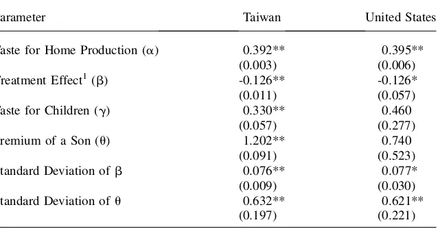
The parameter estimates and their standard errors are reported in Table 5. The es-timate ofais 0.392 in Taiwan and 0.395 in the United States, suggesting that mothers
in Taiwan will on average have a labor force participation rate that is three percentage points lower than in the United States when they have exactly two children. The es-timate ofb, the average treatment effect of a third child on a mother’s labor supply, indicates that a third child would reduce the average mother’s labor supply by roughly 12.6 percent in Taiwan and the United States. Note that the average effect in the two countries is much closer than what is implied by the large difference in the OLS esti-mates for the two countries. The results also indicate that the LATE identified by IV is closer to the model estimate in Taiwan than in the United States.
The difference in the importance of sex preference in fertility decisions between the Taiwan and United States is evident in the parameter estimates. The value of an-other child of the same sexgis 0.33 and 0.46 years of income in Taiwan and the United States respectively, but the premium to having another child of the desired sexuis worth 1.2 years of extra income in Taiwan and only 0.74 years of income in the United States. These estimates should not be interpreted as the true value of a child of the desired sex, since many women have not yet completed fertility.23 However, the results do reflect the larger share of mothers who comply with the in-strument, and does suggest that the Taiwan mothers who are identified by the sex preference LATE may be more representative than those identified for the United States. First, because a large share of mothers is in the group of compliers, they may be more representative of the overall population. Second, because Taiwanese mothers gain a large benefit from a male child, even mothers with high costs of child-bearing may have their fertility decision altered by the instrument. The degree to which parameters are sensitive to who is in the group of compliers is contingent on the degree of heterogeneity (or variance) in the labor supply parameters.
The variance ofbis estimated to be smaller in Taiwan than the United States. For Taiwan, the variance ofbis 0.069, and is 0.089 for the United States, implying that the U.S. population has more heterogeneity than Taiwan’s. The high degree of het-erogeneity inbin the United States creates a situation in which different instruments
Table 4
Comparison of Empirical and Simulated Moments, Taiwan and the United States
Taiwan United States
Actual Simulated Actual Simulated
Panel 1: Comparison of Actual and Simulated Moments
Share having a third child, instrument 0.429 0.435 0.399 0.416 Share having a third child, instrument 0.307 0.308 0.344 0.331 Share working with no child, instrument 0.580 0.604 0.594 0.620 Share working with no child, no instrument 0.587 0.601 0.598 0.614
Share working with child, instrument 0.522 0.505 0.498 0.475
Share working with child, no instrument 0.536 0.516 0.488 0.475
Panel 2: Comparison ofbOLSandbIVin the Actual and Simulated Data
Beta Ordinary Least Squares (bOLS) 20.089 20.093 20.153 20.142
Beta Instrumental Variables (bIV) 20.124 20.111 20.097 20.106
Difference between the estimators (bOLS2bIV) 20.035 20.018 0.055 0.036
Observations 285,172 100,000 304,917 100,000
Source: Taiwan Population and Housing Survey (2000). United States IPUMS 5% (2000). Same sample as in Table 1.
Note: The parameters of the model are chosen by a MATLAB routine minimizing the distance between the empirical moments and simulated moments chosen in panel 1. A measure of the model’s fit is presented in panel 2, in which I compare the reduced form relationships in the data and those observed in the model at the parameter choice. See notes for Tables 2 for a description of the underlying OLS and IV regressions.
970
The
Journal
of
Human
will give very different parameter estimates, since the estimates will be more sensi-tive to who is included in the group of compliers. Only under the ideal situation in which the instrument is affecting mothers around the average values ofaandbwill the local average treatment effect approximate the average treatment effect. In the American context, it may be that a sex-preference instrument will not incorporate these ‘‘high cost’’ mothers, since it is unlikely that the instrument will affect the de-cision of mothers in this region. The degree to which the intensity of sex preference in the two countries accounts for the difference between OLS and IV estimates is ex-plored in the next section.
D. Sex-Preference Intensity and Differences between OLS and IV Estimates
I perform an additional test of this posited relationship between the intensity of an instrument and bIV examining whether subpopulations of mothers with stronger Table 5
Parameter Estimates of the Fertility and Labor Supply Model, Taiwan and the United States
Parameter Taiwan United States
Taste for Home Production (a) 0.392** 0.395**
(0.003) (0.006)
Treatment Effect1(b) -0.126** -0.126*
(0.011) (0.057)
Taste for Children (g) 0.330** 0.460
(0.057) (0.277)
Premium of a Son (u) 1.202** 0.740
(0.091) (0.523)
Standard Deviation ofb 0.076** 0.077*
(0.009) (0.030)
Standard Deviation ofu 0.632** 0.621**
(0.197) (0.221)
*significant at 5 percent. ** significant at 1 percent.
Source: Taiwan Population and Housing Survey (2000). United States IPUMS 5% (2000). Same sample as in Table 1.
Note: The parameters are chosen as the set which minimize the squared difference between the simulated and actual moments of the data (shown in Table 4). The 6 moment conditions allow for identification of the mean of the four model parameters, and the variance of two parameters. The standard deviation of the labor supply paramters (alpha and beta) and the fertility taste parameters (gamma and theta) are restricted to equal the ratio of the parameter means. The model’s parameters can be interpreted relative to the scale in which a fully employed mother earns 10 more years of income than a mother who engages in no market activity, and children impose no direct financial cost. Standard errors are calculated by evaluating the gra-dient of the difference between the simulated and actual moments with respect to changes in the parameter choice. Since 100,000 agents are used for simulation, the standard errors must be increased by a factor equal to (1+1/100000).
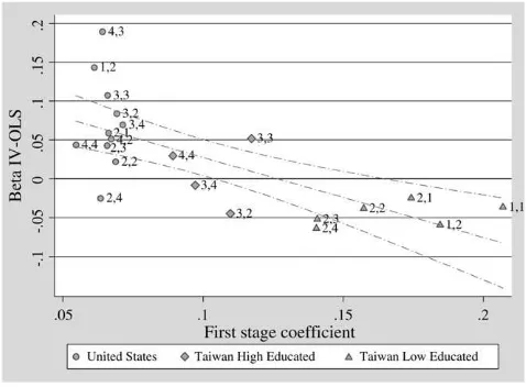
sex preferences withinTaiwan and the United States absorb a larger cost to child-bearing of foregone labor supply. The best measure of son preference in Taiwan’s census data is a mother’s education, and a reasonable proxy for family wealth is the husband’s education. In Figure 2, I estimate separate OLS and IV regressions for subpopulations defined by each combination of husband and wife’s education level, and plot the difference between IV and OLS estimates by the magnitude of the first-stage coefficient (representing the relationship between the sex preference instrument and the probability of a third birth). Figure 2 shows that differences be-tween OLS and IV estimates are negatively related to the magnitude of the first stage. For each subpopulation, OLS estimates are larger in absolute magnitude than IV esti-mates for cells in which the first stage is weak, and IV estiesti-mates are larger in absolute magnitude than OLS estimates for cells in which the first stage is strong. American mothers are clustered in low sex-preference categories, and have smaller labor sup-ply responses.24
Figure 2
Differences between OLS and IV Estimates by Strength of Instrument
Note: Each symbol on the plot above represents a cell composed of parents of a particular education level. The education categories are less than high school (1), high school (2), some college (3), col-lege graduate and beyond (4). Instrument is ‘‘No Son’’ in Taiwan, ‘‘Same sex’’ in the United States. The 14 combinations with fewer than 100 observations (for example, college educated women and men with less than high school) are excluded.
24. An alternative interpretation of this empirical result that bears mention is that the mothers affected by sex preference in Taiwan are not necessarily representative of the overall population. If parents with less education and stronger son preference exhibit lower costs to childbearing, subpopulations with larger first-stage effects will produce more negative IV estimates, but these will not necessarily be closer to the average. Regressions including education as a regressor only change the results slightly, however, suggest-ing that the overrepresentation of low-educated mothers in Taiwan’s IV estimates is not drivsuggest-ing the results. The regression results are available from the author upon request.
The figure reflects that for the United States, the strength of the first stage appears unrelated to the estimates for OLS and IV. One potential explanation is that all the subpopulations exhibit weaker sex preference, and so the instrument is capturing mothers with low costs to childbearing. For Taiwan, however, there is quite a bit of heterogeneity in the intensity of sex preference, allowing for further examination of the relationship between the strength of an instrument andbIV. The figure reflects
that low-educated mothers in Taiwan exhibit intense sex preference and the estimates for IV are larger in absolute value relative to OLS. It also reflects that Taiwan’s more highly educated mothers exhibit an intermediate level of son preference; they exhibit sex preference less intense than less educated Taiwanese women, but more intense sex preference than American women. By examining Taiwan’s highly educated women, one can gauge whether this group with intermediate levels of sex preference also experience an intermediate cost to a child induced by the instrument. Indeed, the results suggest that IV estimates within Taiwan are larger in magnitude when the first-stage coefficient is larger, supporting the claim that instrument intensity and
bIVare related in the way described in the model, where stronger instruments yield
larger estimates of LATE.25
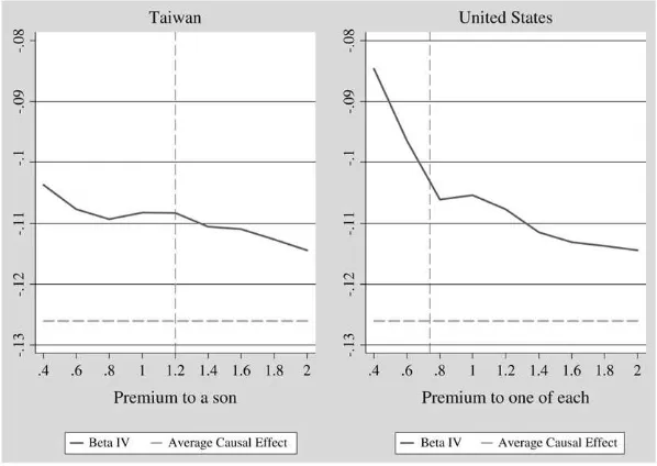
In order to evaluate the relationship between the strength of the sex preference in-strument and the magnitude of IV estimates, I present the results of simulations in Figure 3. The simulations are performed by having the 100,000 randomly drawn agents make fertility decisions using the framework of the model, in reference to each agent’s assigned value of the parameters. For each agent, the parameter values are drawn from a jointly normal distribution which has the covariance structure de-scribed in the previous section. In each simulation I vary the mean premium to hav-ing a child of the desired sex (u), holding the other parameters constant at their optimal values. Following each simulation, I estimatebIVand as reflected in Figure
3, simulations where agents are assigned a higher average value ofuyield more neg-ative values of the local average treatment effect. Note that since the average treat-ment effect of fertility is held constant, the simulations reflect the possibility that LATE may be responsive to the chosen instrument, and stronger instruments may yield better estimates, as they induce even highbimothers into having another child.
IV. Conclusion
In both Taiwan and the United States, I find that the decision to have a third child imposes a large cost to the average mother in foregone labor supply. My results indicate that in Taiwan and the United States, a randomly assigned third child would reduce a mother’s probability of being observed working by roughly 12.6 per-centage points in both countries. The results suggest that a sex preference instrument in Taiwan produces parameter estimates closer to the average treatment effect in the
overall population, possibly owing to the more pervasive nature of son preference in the country. Researchers have attempted to identify the increase in female marital employment that can be explained by declining fertility, and some have cautioned that the correlation between these trends drastically overstates the causal link. My analysis suggests otherwise, and it may be that earlier studies relied on instruments too weak to affect mothers with average costs to childbearing. Recent efforts in Tai-wan to provide cash incentives to childbearing have largely failed, and this may be unsurprising when one considers that many families now rely on the mother’s in-come nearly as much as the father’s.26Policymakers in Taiwan and other low-fertil-ity countries who wish to encourage fertillow-fertil-ity should recognize that additional children imply a longer absence from the workforce for women who have already invested heavily in human capital, and so it may prove more difficult to convince women to have more children than it was to convince them to have fewer children. The results are also important for applied econometricians, since it suggests that even valid instruments may not identify the parameter of interest, especially when the effects of treatment are heterogeneous and parents are able to observe the costs and benefits to treatment.
Figure 3
Simulated Instrumental Variable Estimates by Strength of Instrument
Note: The graphs above show the results of a simulation of the model described in the text. The fig-ures indicate that both in Taiwan and the United States, stronger sex preferences yield IV estimates (solid line) closer to the average causal effect in the population (horizontal dotted line). The vertical line identifies the model estimate of the premium value of the desired sex in each country.
26. online.wsj.com/article_email/SB115578103295937968-lMyQjAxMDE2NTE1NzcxODcxWj.html
References
Angrist, Joshua, and William Evans. 1998. ‘‘Children and their Parents Labor Supply: Evidence from Exogenous Variation in Family Size.’’American Economic Review
88(3):450–77.
Angrist, Joshua. 2004. ‘‘Treatment Heterogeneity in Theory and in Practice.’’Economic Journal114(494):1167–1201.
Bound, John, David Baker, and Regina Baker. 1995. ‘‘Problems with Instrumental Variables When the Correlation Between the Instruments and the Endogenous Explanatory Is Weak.’’
Journal of the American Statistical Association90(430):443–50.
Bronars, Stephen, and Jeff Grogger. 1994. ‘‘The Economic Consequences of Unwed Motherhood: Using Twins as a Natural Experiment.’’American Economic Review
84(5):1141–55.
Card, David. 1999. ‘‘The Causal Effect of Education on Earnings.’’Handbook of Labor Economics,Volume 3, ed. Orley Ashenfelter and David Card. Elsevier Science.
Chamie, Joseph. 2004. ‘‘Low Fertility: Can Governments Make a Difference?’’ Presented at the Population Association of America Annual Meeting, Boston, Mass.
Conley, Dalton, and Rebecca Glauber. 2006. ‘‘Parental Educational Investment and Children’s Academic Risk.’’Journal of Human Resources41(4):722–37.
Cruces, Guillermo, and Sebastian Galiani. 2007. ‘‘Fertility and Female Labor Supply in Latin America: New Causal Evidence.’’Labour Economics14(3):565–73.
Goldin, Claudia. 1995. ‘‘Career and Family: College Women Look to the Past.’’ NBER WP5188.
Heckman, James, and Edward Vytlacil. 2000. ‘‘Local Instrumental Variables.’’ NBER Techinal WP 252.
Imbens, Guido, and Joshua Angrist. 1994.‘‘Identification and Estimation of Local Average Treatment Effects.’’Econometrica62(2):467–75.
Oreopoulos, Philip. 2006. ‘‘Estimating Average and Local Average Treatment Effects of Education When Compulsory Schooling Laws Really Matter.’’American Economic Review
96(1):152–75.
Rosenzweig, Mark, and Kenneth Wolpin. 2000. ‘‘Natural ‘Natural Experiments’ in Economics.’’Journal of Economic Literature38(4):827–74.
Taiwan. Directorate General of Budget, Accounting, and Statistics (DGBAS). Taiwan Population and Housing Census. 2000.
__________. Taiwan Provincial Institute of Family Planning. 2003. Knowledge, Attitudes, and Practice of Contraception in Taiwan (KAP).
__________. Survey of Family Income and Expenditure Survey, Taiwan Area. 1976–2003. United States. IPUMS 5 percent sample 2000. Minneapolis: Minnesota Population Center,
2004.
Westoff, Charles, and Norman Ryder. 1975. National Fertility Survey. ICPSR Study #04334. Willis, Robert. 1973. ‘‘A New Approach to the Economic Theory of Fertility Behavior.’’