1
Modelling On Lecturers‟ Performa
nce
with Hotteling-Harmonic-Fuzzy
1
STH.A
PARHUSIP,
2
NDA.
SETIAWAN
Abstract. This paper is a brief research on modelling of lecturers' performance with modified Hotelling-Fuzzy. The observation data is considered to be as a fuzzy set which is obtained from students survey at Mathematics Department of Science Mathematics Faculty in SWCU in the year 2008-2009.
The modified Hotelling relies on a harmonic mean instead of an arithmetic mean which is normally used in a literature. The used charaterization function is an exponential function which identifies the fuzziness.
The result will be a general measurement of lecturers' performance. Based on the 4 variables used in the analysis (Utilizes content scope and sequence planning, Clearness of assignments and evaluations, Systematical in lecturing, and Encourages students attendance) we obtain that lecturers' performance are fair, poor, fair, and poor respectively.
Keywords and Phrases : Hotelling, harmonic mean, fuzzy, exponential function, characteristic function.
1. INTRODUCTION
University is one of post investments for human development in education which most activities based on the learning process during in a university. This process relies on interaction between lecturers and students. After some period of time, students may adopt some knowledge which may determine their futures. Therefore lecturers require to transfer their knowledge such that students capable to reproduce their knowledge obtained in their universities as a support for themselves in their working places.
Since a lecturer becomes an important agent in the effort of human development in a university, some necessary conditions must be satisfied as a lecturer. This paper will propose some results on lecturers' performance based on students survey. Students evaluate a lecturer by some questions (some are adopted from a literature given in a web which are listed on Table 1 and these are considered the same items in Indonesian that have been used as instruments in the observation for this paper.
According to Yusrizal [1], the items are validated which is not done in this paper. We have used these items to evaluate lecturers‟ performance. Each item will be quantified as 0, 1, 2 or 3 which means poor, fair, satisfactory and good respectively. Since all students did not meet with all lecturers in 1 semester then the research is simply made as a general evaluation for all lecturers in the Department.
________________________________
The used data here are obtained from students survey in Mathematics Department in Science and Mathematics Faculty, Satya Wacana Christian University in the year 2008-2009. Furthermore, the lecturers‟ performance can not be exactly in one of the values 0,1, 2 or 3. Therefore data can be considered nonprecise and hence we refer to fuzzy in presenting the analysis.
The remaining paper is organized as follows. The used theoretical background is shown in Section 2. Procedures to analyze the obtained data are shown on Section 3. The analysis is then shown in Section 4 and finally some conclusion and remark are written in the last Section of this paper.
II. MODELLINGHOTELLING-HARMONIC-FUZZY
ONLECTURERS’PERFORMANCE
2.1 Review Stage
Some authors have proposed a quality evaluation based on some mathematical approaches such as using fuzzy set. Teacher performance is studied with fuzzy system [2] to generate an assesment criteria. In complex system such as cooling process of a metal, the combined PCA (Principal Component Analysis) algorithm and T2-Hotteling are used to define quality index after all data are normalized in a range -1 and 1 [3]. The other instrument
for lecturers‟ performance have been developed and validitated using variable
analysis . Lecturers‟ strictness are also estimated using intuitionistic fuzzy [4]. There are several standards can also be used to indicate a quality of a teacher which are more a qualitative approach which are easily found through internet. In a strategic planning, SWOT is one of the most pointed references. In SWOT analysis some uncertainties can be encountered and therefore using fuzzy will renew the classical SWOT by presenting the internal and external variables in
TABLEI
QUESTIONS FOR STUDENTS OBSERVATION TO EVALUATE A LECTURER HELD DURING
IN A CLASS
No Questions
1 Utilizes content scope and sequence planning
2 Clearness of assignments and evaluations
3 Systematical in lecturing
4 Encourages students attendance
5 Demonstrates accurate and current knowledge in subject field
6 Creates and maintains an environment that supports learning
7 Clearness to answer the question from a student
8 Attractiveness of the lecture
9 Clearness of purpose on each assignment
10 Lecturer‟s competence on stimulating students excitement 11 Lecturer‟s competence on delivering idea
12
Does teacher have available time to help students for the related topic outside the class?
13 Effectiveness of time used in the class
14 Provides relevant examples and demonstrations to illustrate concepts a
the sense of fuzzy as shown by Ghazinoory, et.all[5].
It is assumed that the given data contain non-precision. Thus the representation data will be as a fuzzy set [6]. The fuzzy data are indicated by a characteristic function. There are some well-known characteristic functions. In this research, we apply an exponential characteristic function ,i.e
2 2 1 1 ), ( , 1 ), ( ) ( m x x R m x m m x x L x
with
1 1 1 exp ) ( q a m x x
L and
2 2 2 exp ) ( q a m x x R
. (1)
There are 6 parameters in Eq.(1), i.e m1,a1,q1 and m2,a2,q2 that must be
[image:3.612.132.478.135.192.2]determined. An illustration of this characteristic function is depicted in Figure 1. Figure 1 shows us that a single value x*=0.5 can be considered that the value may vary in the interval 0.25x*1.5. This allows us to tolerate that the given value is not exactly 0.5 but it can be in this interval which indicates its non-precision. However, if this tolerance is too big, one introduces a parameter
which varies in 01 such that our tolerance can be chosen freely. For example, if 0.2 then the tolerance for saying 0.25x*1.5 is reduced asillustrated in Figure 1. We may say that 0.35x*0.85.
Fig 1.
(x) with the given data is 0.5 (denoted by star on the peak) , and the value of eachparameter m1
,
a1,
q1is 0.4980, 0.1 , 2 respectively and the value of each parameter m2,a2,q2 is 0.2, 0.502 , 0.8 respectively. The tolerance for x* is reduced. The corresponding cutis also shown as a horizontal line for 0.2.A problem appears here that the determination of parameters becomes time consuming for each value. Up to now, there exists no optimization procedure to find the best values of parameters here. Therefore we may vary parameters based on the given data. Let us consider by this following example.
Example 1: Let the given data be a vector x [0.5 0.67 0.83 1. 1.17 1.33 1.5 1.67 1.83 2]T. Let the vector x be an element in the observation space
X
M . We want to express this vector in the sense of fuzzy. By trial and error we try to use the value of each parameter. This means that each value in the vector has its own characteristic function. We will also define the average value of this vector by the harmonic mean and the characteristic function of this average value. The used parameters for all characteristic functions are
2 ,
1 . 0 1 2
1 q q
a ,a20.2. These parameters are chosen freely. The illustration of characteristic functions is depicted in Figure 2a. The values of m1 and m2 are taken from the given vector. The characteristic function of the harmonic average is obtained as
309 . 1 ), ( 039 . 1 , 1 039 . 1 ), ( ) ( x x R x x x L x
with
2 1 . 0 039 . 1 exp )
(x x
[image:3.612.236.378.318.410.2]
2
2 . 0
039 . 1 exp
)
(x x
R .
Thus the characteristic function is defined after the harmonic mean is obtained. The statistical test for multivariate data is based on the T2 named as Hotelling [7] in a classical sense that
1( 0)0
2
nX TS X
(2)
whereX
(
x1,
x2,
...,
xp)
T is a vector of an arithmetic mean of eachvariable,
n
i ki
k x
n x
1
1 is an arithmetic mean for the k-th item. It is also
known from Wikipedia or [7] that
2 1 , 2~
n p T
or
p n p
F n
p p n
, 2
~ ) 1
(
[image:4.612.145.423.309.615.2]. (3)
Fig 2 The illustration of all characteristic functions with a1
,
q1 are 0.1 and 2. and a2, q2are 0.2 and 2.The value of m1 and m2 are taken from the given vector.Since
2 is distributed as) ( ) (
) 1 (
,n p p F p n
p n
, then
2 can be used for hypotheses. Atest of hypothesis: H0:0versus H1:0 at the level of significance, reject H0 in favor of H1 if [7]
) ( ) (
) 1 (
,
2
Fpnp
p n
p n
. (4)
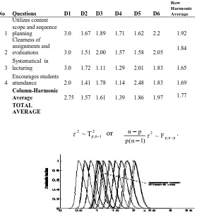
TABLE II
STUDENTS SURVEY FOR 6 LECTURERS BASED ON 4 VARIABLES
THE SYMBOL DjINDICATES THE NAME OF J-TH LECTURER.
No Questions D1 D2 D3 D4 D5 D6
Row Harmonic Average
1
Utilizes content scope and sequence
planning 3.0 1.67 1.89 1.71 1.62 2.2 1.92
2
Clearness of assignments and
evaluations 3.0 1.51 2.00 1.57 1.58 2.05 1.84
3
Systematical in
lecturing 3.0 1.72 1.11 1.29 2.01 1.83 1.65
4
Encourages students
attendance 2.0 1.41 1.78 1.14 2.48 1.83 1.69
Column-Harmonic
Average 2.75 1.57 1.61 1.39 1.86 1.97 1.77
[image:4.612.137.433.310.616.2]Thus the control limit of the
2control chart can be formed as [8] ) ( ) ( ) 1 (,n p p F p n p n UCL
and LCL=0. (5)
There is a reason proposed in [8] for LCL=0 , but it ignores here. It is convenient to refer to the simultaneous intervals for the confident interval of each j,
j=1,…,p as ([7](page 193))
j x n s F p n p n x n s F p n p n jj p n p j j jj p n
p ( )
) ( ) 1 ( ) ( ) ( ) 1 ( , ,
, j=1,…,p.
Equation (5) allows us to simplify the statement above as
n s UCL x n s UCL
xj jj j j jj , j =1,…,p. (6)
In this paper, we will replace an arithmetic mean by a harmonic mean in the sense of fuzzy. The harmonic mean is used to increase the precision of average quantity (since we know that arithmetic mean ≥ harmonic mean) and the harmonic mean is formulated as
n i i H x n x 1 1
The harmonic mean will be useful if we have highly oscillated data. Additionally, there exists no literature so far in doing this way which shows an originality of this paper though the number of the used data is considerable small. The used covariance matrix S is in the usual way, i.e
p p p p p p S S S S S S S S S S , 2 , 1 , , 2 22 21 , 1 12 11 .... ... .... .... .... ...
... with
n i q qi p pipq x x x x
n S 1 ) )( ( 1
for p, q = 1, 2, ...., M.
The example 2 shows the idea of Hotteling-harmonic-Fuzzy. Note that the number of samples for each item (variable) is 6.
Example 2. Suppose the given data are shown in Table 2 with each number in the entry is an average from the nj-number of students for each lecturer. We assume that the result is independent with the number of students in each class. If each number in the Table 2 presented as a characteristic function then there will be many parameters must be determined. Hence we define the characteristic function of the harmonic mean of each item. The resulting of characteristic-harmonic mean is depicted in Figure 2.
Furthermore, the harmonic mean of each lecturer in the whole items and for each item for all lecturers are shown in Table 2. Based on the average quantity, one has 1.77 which is not precisely in the original values (0, 1, 2, and 3). Since it
closes to 2, the lecturers‟ performance is considered satisfactory. This paper will
evaluate into more rigorously.
The covariance matrix in the classical sense can be obtained by function cov in MATLAB, one yields
0.2422 0.2008 0.1185 0.0939 0.2008 0.4447 0.2759 0.2748 0.1185 0.2759 0.3180 0.2921 0.0939 0.2748 0.2921 0.2776 S
matrix covariance sample Shis obtained as 0.2157 0.1881 0.1114 0.0889 0.1881 0.4015 0.2488 0.2449 0.1114 0.2488 0.2765 0.2531 0.0889 0.2449 0.2531 0.2396 h S
. In the
rest paragraphs we will compute all related formulas using harmonic mean.
One may also observe that covariance matrix Shis positive definite by computing its eigenvalues which are all positive (0.0015, 0.0717, 0.1710 and 0.8891).We have also compute the invers matrix of Sh as
2192 . 19 9823 . 15 7142 . 54 0196 . 67 9823 . 15 4292 . 20 3587 . 53 3350 . 71 7142 . 54 3587 . 53 6743 . 274 4680 . 324 0196 . 67 335 . 71 4680 . 324 0665 . 395 1 h S
. Finally one needs to consider the
Hotelling to involve in this paper which mostly taken from literature (Johnson and Wichern, 2007) and reformulate it using harmonic mean.
The hypothesis test withH0
:
T1 , 2 , 2 , 3 0
against H1
:
T1 , 2 , 2 , 3 1 at
level significance0.10is employed here. The observed
2 is
2=238.9666.Comparing the observed 2=238.9666 with the critical value (using Eq.4)
(0.10)
2 ) 4 ( 5 ) 10 . 0 ( ) ( ) 1 ( 2 , 4 , F F p n p n p n p 10(9.2434)=92.434.
Thus we get
2> 92.434 and consequently we rejectH0 at the 10% level of significance. For completeness, The value ofF4,2(0.10) is computed using function in MATLAB and type as finv(0.90,4,2). Finally, we try fuzziness takes place in this hypothesis.2.2 Hotelling-fuzzy
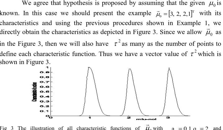
We agree that hypothesis is proposed by assuming that the given
0is known. In this case we should present the example
T1 , 2 , 2 , 3 0
with its
characteristics and using the previous procedures shown in Example 1, we directly obtain the characteristics as depicted in Figure 3. Since we allow
0
as in the Figure 3, then we will also have
2as many as the number of points to define each characteristic function. Thus we have a vector value of
2which is shown in Figure 3.Fig 3 The illustration of all characteristic functions of
0with a10.1,q12 and2 , 2 .
0 2
2 q
a . The values of m1 and m2 are taken from the harmonic mean of each item on Table 2. Note that there exists 4 characteristic functions but the second and the third are in the same curves.
Be aware that the given 0
[image:6.612.128.487.445.655.2]index of each characteristics function (since each function is discritized) and hence find the corresponded value of x. What will be a problem here ?. We need always a set of
0 (with the number of element is the same as the predicted one) . Let us study for (x)= 0.6 for one of possible memberships of 0. We draw ahorizontal line that denotes (x)= 0.6 to find intersection points such that we can
draw the vertical line (denoted by an arrow in Figure 4).
The vertical lines denote the possible new sets of 0and we always have two values of each given characteristic value (membership) that may act as the bounds of each fuzzy-0 . Let us denote these intervals as j
o
I , where index j
denotes the j-th vector of 0
. Thus to make the computation simpler, we choose the inf( j
o
I , ) and sup(Io,j
) to continue our hypothesis. The used number of
points will influence the obtained fuzzy-0.
Fig 4 The illustration of all 0taken from the characteristic function with a10.1,q12 and a20.2,q22. The values of m1 and m2 are taken from the harmonic mean of each item on Table 2.
Due to numerical techniques, the idea to use the inf( j
o
I , ) and sup(Io,j) still
can not be implemented. Instead, we can do manually, but it will be time consuming if we have a large number of points. Thus we are left this problem for the next research. In this paper we apply
0 in the hypothesis as the usual procedure in a classical sense.Example 3. Suppose that we have
T1 , 2 , 2 , 3
0
and the resulting characteristic function is shown in Figure 4. If (x)=0.6, we get intervals of each value of
T1 , 2 , 2 , 3
0
as shown in Figure 4. Practically, there exists no
(
x)
=0.6 precisely since its value is constructed by Equation 1. Manually, by drawing the horizontal line and the vertical line as shown in Figure 4, we have approximations of inf( jo
I , ) and sup(
j
o
I , ). We propose that inf(
j
o
I , )=[0.8,
1.9, 1.9, 2.9] and sup(Io,j).=[1.1, 2.1, 2.1, 3.2]. These results lead to the same
conclusion that H0
:
T1 , 2 , 2 , 3
0
is again rejected at the 10% level of significance.
On the other hand, one may determine all sets of 0to find a
100%(1-
) confidence region for the mean of a p-dimensional normal distribution such that
( 0)1 0
2
nX TS X
) ( ) (
) 1 (
,np p
F p n
p n
(7)
[image:7.612.130.459.189.347.2]necessary.
III.RESEARCHMETHOD
The used data are taken from the students‟ survey. We assume that the observations are independent with the given lecturers and the number of students on each class. Table 1 contains questions which are used to evaluate lecturers‟ performance. The result is shown in Table 3.
3.2 Calculate harmonic mean of variable
The harmonic mean of each variable is computed using formula in Section 2. 3.3 Covariance matrix is computed which its average formula is taken from the harmonic mean. If the covariance matrix is singular, one needs to reduce the number of variables by principal component analysis.
3.4 Given the predicted 0 then define the characteristic function of each element of
0
.
3.5 Compute the value of 2for each set of 0
taken from the characteristic function.
IV.RESULTANDANALYSIS
Evaluation is based on Table 2 which means that we have p=16 as the number of variables. Unfortunately, the covariance matrix is almost singular that causes the invers matrix is badly obtained. One may observe by computing its determinant which tends to 0 (O( 170
10 )). According to [7](page 110), this is caused by the number of samples is less than the number of variables which happens in any samples. This means that some variables should be removed from the study. The corresponding reduced data matrix will then lead to a covariance matrix of full rank and nonzero generalized variance. Thus as
TABLEIII
STUDENTS SURVEY FOR 6 LECTURERS BASED ON 16 VARIABLES
THE SYMBOL DjINDICATES THE NAME OF J-TH LECTURER.
No D1 D2 D3 D4 D5 D6
1 4.00 2.67 2.89 2.71 2.62 3.20
2 4.00 2.51 3.00 2.57 2.58 3.05
3 4.00 2.72 2.11 2.29 3.01 2.83
4 3.20 2.41 2.78 2.14 3.48 2.83
5 4.00 2.59 2.11 2.29 3.14 2.88
6 3.20 2.79 2.89 2.29 3.48 2.85
7 4.00 2.41 3.11 2.43 3.35 3.12
8 3.73 2.33 2.33 2.14 2.88 2.67
9 4.00 2.21 3.00 2.71 2.75 3.02
10 3.73 2.33 2.89 2.29 2.67 3.03
11 3.73 2.62 3.00 2.71 3.40 2.92
12 4.00 2.31 2.56 2.86 3.18 2.43
13 3.47 2.51 3.56 2.86 3.05 3.38
14 3.47 2.23 3.22 2.71 3.05 3.20
15 3.73 2.36 3.11 2.29 2.92 2.92
mention in Section 2, we need to use principal components analysis (PCA). The standard PCA was employed, we compute the proportion of total variance accounted by the first principal component is
p jj 1
1
= 0.7943.
Continuing, the first two components accounted for a proportion
pj j 1
2 1
=
0.8933 of the sample variance. After the sixth eigenvalue, we observe that only six variables with nonzero proportions. Thus we will only consider the 6 variables in the analysis. Additionally, we also observe that
j 0,j=7,…,p whereas
1
3.1702,
2
0.3948,
3
0.2859,
4
0.1110,
5
0.0274, and
6
0.0016. It is reasonable to choose the first six variables. Unfortunately, the singular covariance matrix still exists. To handle this problem, the pseudo-invers matrix is applied. Again, one needs to concern Equation (2) that the number of samples is not allowed to be the same as the number of variables which leads to the division by zero. Since the eigenvalues represent variables variances, we select only the first four variables such that n > p. In this case, we are led to the result in Section 2.The control limit of the
2control chart can be obtained by using Eq.(4), one yields) 10 . 0 ( ) 4 6 (
4 ) 1 2 (
2 , 4
F UCL
= 92.4342 and LCL=0.
Section 2 suggests us to compute the confidence intervals of the reduced data and we have the following results
8552
.
4
0453
.
1
1
; 0.8337
2 4.9181; 1428. 5 2776
.
0
3 ; 0.94654 4.5201.Up to now, the conclusion for lecturers‟ performance qualitatively is not
yet concluded which is practically useful for application. These intervals show us that all observed values are in the intervals. Finally, we suggest that the evaluation is proceeded as follows :
1. Compute the UCL= ( )
) (
) 1 (
,n p p
F p n
p n
, n= the number of the observed
lecturers, p = the number of variables used in the evaluation (the number of items used to survey).
2. Compute the harmonic mean of each variable.
3. Compute the interval confidence of harmonic mean of each variable using the Equation (6).
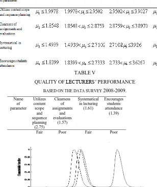
TABLE IV
INTERVAL CONFIDENCE FOR EACH VARIABLE
VS EACH QUALITY OF LECTURERS‟ PERFORMANCE
TABLE V
QUALITY OF LECTURERS‟ PERFORMANCE
BASED ON THE DATA SURVEY 2008-2009.
Name of parameter
Utilizes content scope
and sequence planning (2.75)
Clearness of assignments
and evaluations
(1.57)
Systematical in lecturing
(1.61)
Encourages students attendance
(1.39)
[image:10.612.148.456.148.515.2]Fair Poor Fair Poor
Fig 5 Characteristic function of each subinterval of
1
.
V. CONCLUSION
This paper proposes an evaluation of lecturers‟ performance by Hotelling
-harmonic-fuzzy. The harmonic mean is used to increase the precision of averaging and replace the arithmetic mean in the covariance matrix. The Hotelling is employed here to find the confidence interval of mean value of each variable. Using 16 variables, we obtain singular covariance matrix such that only 4 variables must be considered in the analysis through principal component analysis and we must have the number of variables (p) must be less than the number of observations (n).
The studied data are the students‟ survey in Mathematics Department of Science and Mathematics Faculty, Satya Wacana Christian University in the year 2008-2009. Based on the 4 variables used in the analysis, we obtain that
[image:10.612.160.430.321.525.2]Acknowledgement. The authors gratefully acknowledge T. Mahatma,SPd,
M.Kom for assistance with English in this manuscript, and the Research Center in Satya Wacana Christian University for financial support of this work.
References
[1] Yusrizal and Halim, A.,”Development and Validation of an Intrument to
Access the Lecturers‟ Performance in the Education and Teaching Duties”,
Jurnal Pendidikan Malaysia 34(2) 33-47,2009.
[2] Jian Ma and Zhou, D. „‟Fuzzy Set Approach to the Assessment of Student-Centered Learning‟‟, IEEE Transaction on Education, Vo. 43, No. 2,2000. [3] Bouhouche, S., Bouhouche, M. Lahreche, , A. Moussaoui, and J. Bast,
„‟Quality Monitoring Using Principal Component Analysis and Fuzzy Logic Application in Continuous Casting Process‟‟, American Journal of Applied Sciences, 4 (9):637-644,ISSN 1546-9239, 2007.
[4] Shannon, A, E. Sotirova, K. Atanassov, M. Krawczak, P.M, Pinto, T. Kim,
„‟Generalized Net Model of Lecturers‟s Evaluation of Student Work With
Intuitionistic Fuzzy Estimations‟‟, Second International Workshop on IFSs Banska Bystrica, Slovakia, NIFS 12,4,22-28,2006.
[5] Ghazinoory, A., Zadeh, A.E., “Memariani, Fuzzy SWOT analysis, Journal of Intelligent & Fuzzy Systems” 18, 99-108, IOP Press, 2007.
[6] Viertl, R., “Statistical Methods for Non-Precise Data”, CRC Press,Tokyo, 1996.
[7] Johnson, R.A. and Wichern,D.W Applied Multivariate Statistical Analysis, 6th ed. Prentice Hall, ISBN 0-13-187715-1, 2007.
[8] Khalidi, M.S.A, „‟Multivariate Quality Control, Statistical Performance and Economic Feasibility‟‟, Dissertation, Wichita State University, Wichita-Kansas ,2007.
HANNA ARINI PARHUSIP
: FSM-SATYA WACANA CHRISTIAN UNIVERSITY.E-mails: [email protected]
ADI SETIAWAN
: FSM-SATYA WACANA CHRISTIAN UNIVERSITY.