Full Terms & Conditions of access and use can be found at
http://www.tandfonline.com/action/journalInformation?journalCode=ubes20
Download by: [Universitas Maritim Raja Ali Haji] Date: 11 January 2016, At: 23:00
Journal of Business & Economic Statistics
ISSN: 0735-0015 (Print) 1537-2707 (Online) Journal homepage: http://www.tandfonline.com/loi/ubes20
Nonparametric Estimation of Labor Supply and
Demand Factors
Tsunao Okumura
To cite this article: Tsunao Okumura (2011) Nonparametric Estimation of Labor Supply and
Demand Factors, Journal of Business & Economic Statistics, 29:1, 174-185, DOI: 10.1198/ jbes.2010.08068
To link to this article: http://dx.doi.org/10.1198/jbes.2010.08068
© 2011 American Statistical Association
Published online: 01 Jan 2012.
Submit your article to this journal
Article views: 364
Nonparametric Estimation of Labor Supply
and Demand Factors
Tsunao OKUMURA
International Graduate School of Social Sciences, Yokohama National University, Yokohama 240-8501, Japan (okumura@ynu.ac.jp)
This article derives sharp bounds on labor supply and demand shift variables within a nonparametric simultaneous equations model using only observations of the intersection of upward sloping supply curves and downward sloping demand curves. Furthermore, I demonstrate that these bounds tighten with the imposition of plausible assumptions on the distribution of the disturbance terms. Using Katz and Murphy’s (1992) panel data on wages and labor inputs, I estimate these bounds and assess the supply and demand factors that determine changes within male–female wage differentials and the college wage premium.
KEY WORDS: College wage premium; Gender wage differentials; Panel data model; Partial identifica-tion; Sharp bound; Simultaneous equations.
1. INTRODUCTION
Simultaneous equations models of supply and demand pro-vide a useful framework for the analysis of changes in wage structure. The seminal works of Katz and Murphy (1992) and Murphy and Welch (1992) demonstrated the utility of this framework by assessing what supply and demand factors cause changes in gender and educational wage differentials. However, these works only observed the equilibrium wages and labor in-puts (i.e., the intersections of the labor supply and demand func-tions) and hence failed to identify the supply and demand fac-tors. Naturally, this raises to the question of what can be identi-fied from the data alone.
This article estimates sharp bounds on supply and demand shift variables within a nonparametric simultaneous equations model. The analysis requires only observations of the intersec-tions of the upward sloping supply and downward sloping de-mand curves (wages and labor inputs); it is not necessary to specify supply and demand functional forms or the distribu-tion of disturbances. Such an approach mitigates possible prob-lems relating to model misspecification and nonidentification by asking what can one infer about shift variables within a non-parametric simultaneous equations model using only weak and credible assumptions.
To introduce the intuition behind the bounds, consider the following model:
q
it=fit(pit)+μt+εit (supply),
qit=git(pit)+νt+ξit (demand),
(1)
where i indexes the gender/educational/skill group,t indexes time,qitis the growth rate of labor inputs, andpitis the growth
rate of real wages. μt denotes a supply shift variable and νt
is a demand shift variable, which are fixed time effects. I will assume thatfit(·)is an increasing function,git(·)is a
decreas-ing function, andfit(pit)=git(pit)=qit for (qit,pit),which is
known.εit andξit are disturbances and their medians foriare
zero. Imagine a figure in which the horizontal axis represents
qit, the vertical axis represents pit, and(qit,pit)is the origin.
In period t, when most of the cross-section observations are found in the southeast region to the lower right of(qit,pit), it
is likely that the supply shift variableμt is positive.
Symmet-rically, when most observations are found in the northwest re-gion to the upper left of(qit,pit), it is likely thatμtis negative.
I use this intuition to demonstrate that the supply-side shift vari-ableμt is identified within bounds. The case for the
demand-side shift variableνtis handled symmetrically.
These bounds can be narrowed by introducing additional as-sumptions on the distributions of the disturbancesεit andξit.
This article considers the following restrictions: (1) the distur-bances are symmetric about zero and (2) the distribution of the disturbances are known. Analyzing the data used by Katz and Murphy (1992), I estimate supply and demand shift variables for each of their gender and educational categories. From these estimates of the sharp bounds, I discuss how the shifts in the demand and supply factors caused changes within the male– female wage differentials and the college wage premium within the United States.
Katz and Murphy (1992) argued that when most of the growth in labor inputs and real wages(qit,pit)are found in the
southeast and northwest regions (e.g., in the 1970s), supply shift is a relatively important component of the changes in wages and labor inputs; however, when most of the growth is found in the northeast and southwest regions (e.g., in the 1980s), de-mand shift is a relatively important component. Katz and Mur-phy (1992) examined these relationships by investigating the signs of the inner products between changes in wages and la-bor inputs. In contrast, consider the following approach: (1) ob-serve that if(qit,pit)is in the southeast region to the lower right
of(qit+α,pit), then this is a sufficient condition forμt+εit
to be greater thanα(since supply curves are upward sloping) and (2) observe that if (qit,pit)is in the northeast, southeast,
and southwest regions as compared to(qit+α,pit), then this
is a necessary condition forμt+εit to be greater thanα. The
probability thatμt+εitis greater thanαis bounded above and
below by the probabilities of these two events. Therefore, the distribution ofμt+εit [which equals 1−P(μt+εit> α)] is
identified within bounds. By assuming the median ofεitforiis
zero, these bounds will translate into restrictions on the supply shift variableμt, which will be shown to be identified within
bounds. The symmetric result holds for the demand shift vari-ableνt.
The econometric methodology of this article follows in the tradition of Manski (1997) and Manski and Pepper (2000). Under the weak assumption of monotone treatment response, Manski (1997) derived sharp bounds on functionals of the dis-tribution of treatment response that respect stochastic domi-nance. In particular, corollaryM1.3 in Manski (1997) identified the bounds on the quantiles of the treatment response function
y(t) as a special case. Though this article is similar to Man-ski (1997) in spirit, as both embrace inference under weak and credible assumptions, in order to estimate labor supply and de-mand shift variables, I derive sharp bounds on the median of the disturbances that generate the distribution of the outcomey(t).
There is a large and recent literature that examines the identification of nonparametric simultaneous equations models (see Matzkin2007for a survey). Within this literature, Brown and Matzkin (1998), Ekeland, Heckman, and Nesheim (2004), and Matzkin (2008) studied nonparametric identification of the supply and demand system without assuming a triangular sys-tem. Their work took into consideration that both supply and demand functions can arise from the aggregation of heteroge-neous individual behavior, which corresponds toμt+εit and
νt+ξitwithin the current framework. Rigobon (2003) and
Lew-bel (2008) used disaggregate heterogeneous individual behavior to examine the identification of parametric simultaneous equa-tions models. Recently, there is a growing literature on the ap-plication of Manski’s (1994,1997) and Manski and Pepper’s (2000) bounds to labor markets. Blundell et al. (2007) estimated the distribution of wages in the United Kingdom using these bounds, using selection-into-work as a treatment variable.
This article is organized as follows. Section2discusses the econometric model. Section3 estimates the labor supply and demand shift variables by employing panel data on labor inputs and wages in the United States. Section4concludes.
2. SHARP BOUNDS ON THE MEDIAN OF DISTURBANCES WITHIN THE SUPPLY
AND DEMAND FRAMEWORK
In preparation to estimate supply and demand shift variables I begin by setting up a simultaneous equations model with two endogenous variables and two disturbances. The objective is to estimate the medians of the disturbances:
q=f(p)+u,
q=g(p)+v, (2)
wherepandq are endogenous variables andu andvare dis-turbances. The population is formalized as a measure space(J, ,P)of agents, withPa probability measure. ThenP[(u,v), (q′,p′)]gives the distribution of disturbances and realized vari-ables.f(·)andg(·)are an increasing and a decreasing function ofp, respectively.p andumay be correlated, asp andvalso may be. The solution (q,p) of Equation (2) is unique, given
(u,v).
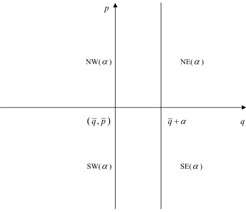
Figure 1. NE(α),SE(α),NW(α),and SW(α)represent the north-east, southnorth-east, northwest, and southwest regions of the point,
(q+α,p), respectively, for some real number α and (q,p), where f(p)=g(p)=q.
I take the existence of a known point(q,p)such thatf(p)=
g(p)=q as prior knowledge. As Figure 1illustrates, NE(α),
SE(α), NW(α), and SW(α) represent the northeast {(q,p)|
q>q+α,p>p}, southeast{(q,p)|q>q+α,p≤p}, north-west {(q,p)|q≤q+α,p>p}, and southwest {(q,p)|q≤
q+α,p≤p}regions of(q+α,p), respectively, for some real numberα. Suppose that(q,p)is observed in SE(α). Since the
f function is upward sloping,u (measured at theq-axis inter-sected by thef function) is greater thanα. In contrast, if(q,p)
is observed in NW(α),uis smaller thanα. This relation implies the following proposition.
Proposition 1. Suppose Equation (2). For any real numberα, (i) P((q,p)∈NW(α))
≤Fu(α)≤1−P((q,p)∈SE(α)), (3)
(ii) P((q,p)∈SW(α))
≤Fv(α)≤1−P((q,p)∈NE(α)), (4)
whereFu andFv are the cumulative distribution functions of
the disturbancesuandv, respectively. These bounds are sharp.
Proof. SeeAppendix A.
Proposition1shows that the distribution of the observations
(q,p)reveals the distributions of the disturbancesuandvup to bounds because both bounds in Equations (3) and (4) weakly increase inα. These bounds hold for arbitrary correlations be-tweenuandp, as well as those betweenvandp. For any real number α, the bounds on Fu(α) and Fv(α) are estimated by
using the analogy principle by replacing population quantities with their empirical counterparts.
The quantiles ofFuandFv are restricted by the quantiles of
the bound estimates onFuandFv, respectively. Specifically, the
medians ofuandv, which are denoted byuandv, are bounded by the medians of the bound estimates onFuandFv.
Lemma 1. Define:
These bounds are sharp.uandvare bounded on one side; they are never bounded on both sides, however.
Proof. SeeAppendix B.
If more (less) than a half portion of(q,p)’s are distributed in the region wherepis greater thanp, then the upper (lower) bounds onuand the lower (upper) bounds onvexist; the oppo-site bounds do not exist, however.
Manski (1997) presented sharp bounds on the quantiles of the weakly increasing functiony(t)at some treatmenttby ob-serving the realized treatment and the realized outcome (corol-laryM1.3). Let us suppose thatyj(·)is specified asfj(·)+uj(·),
and fj(t)is known; then, the sharp bounds on the median of
uj(t)are attained by the median ofyj(t)−fj(t), the difference
between treatment response and the known value offj(t).
Introducing certain assumptions narrows the sharp bounds of the disturbances’ medians. The following two assumptions about the distributions ofuandvare considered.
Assumption 1. The distributions of u andv are symmetric around the medians ofuandv, respectively.
Assumption 2. Fu is defined as the distribution of u−u,
whereu is the median ofu.Fv is defined as the distribution
ofv−v,wherevis the median ofv. Let us assume that (1)Fu
andFvare known by an econometrician and (2)FuandFv are
strictly increasing functions.
The locations of individual supply and demand curves (mea-sured atqwhenp=p) are characterized by supply and demand disturbances. Assumption 1, therefore, supposes that individ-ual curves are symmetrically located with respect tou andv. Assumption2demonstrates that the distributions of individual disturbances are known up to a location parameter (uorv), as a semi-parametric approach assumes.
Lemma 2. Assume Assumption1. Define:
α1(γ )=infα|P[(q,p)∈NW(α)] ≥γ,
These bounds are sharp. These bounds are tighter than or equal to those in Lemma1.uandvare bounded on one side; they are never bounded on both sides, however. Under Assumption1, the unbounded sides ofuandvin Lemma1are not bounded.
Proof. SeeAppendix C.
Lemma 3. Assume Assumption2. Then sup
Assumption1has identifying power in that it can tighten the bounds onuandv. Assumption1, however, cannot identify the unbounded sides ofuandvin Lemma1. In contrast, by impos-ing Assumption2,uandvare bounded on both sides.
In Equation (2), I assume that the supply and demand func-tions are additively separable. By relaxing this assumption, I can generalize the above results to functions that appear in a nonseparable form in the simultaneous equations model:
be correlated. Equation (2) is the case of Equation (10) under Assumptions3,4, and5.
Define NE∗(α)= {(q,p)|q>f∗(p, α),p>p}; SE∗(α)= {(q,p)|q>f∗(p, α),p≤p}; NW∗(α)= {(q,p)|q≤f∗(p, α),
p>p}; and SW∗(α)= {(q,p)|q≤f∗(p, α),p≤p}.
The following sharp bounds on the distributions ofu andv
are obtained.
Proposition 2. Suppose Equation (10) and Assumptions3,4,
whereFu andFv are the cumulative distribution functions of
the disturbancesuandv, respectively. These bounds are sharp.
Proof. SeeAppendix E.
3. ESTIMATION OF LABOR SUPPLY AND DEMAND SHIFT VARIABLES
Equation (2) is modified using the following panel data model:
q
it=fit(pit)+μt+εit,
qit=git(pit)+νt+ξit,
(12)
whereiis the gender/educational/skill group index andtis the time index.qit andpit are the growth rates of the labor inputs
and real wages of theith group at timet.(qit,pit)is a
normal-ization satisfyingfit(pit)=git(pit)=qit.fit(·)andgit(·)are
in-creasing and dein-creasing functions, respectively.μt andνt are
supply and demand shift variables and unknown parameters (fixed time effects) to be estimated. εit and ξit represent
dis-turbances with supply and demand functions and the medians ofεitandξitforiare zero.μt+εitandνt+ξitcorrespond tou
andvin Equation (2), and thus,μtandνtcorrespond touandv.
This model posits that the growth rates of labor supply and wages comove across groups because of the change in the sup-ply and demand shift variables (μt andνt). Yet, this
comove-ment is not deterministic as independent movecomove-ment is caused by idiosyncratic supply and demand disturbances (εit andξit).
Supply and demand curves,fit(·)andgit(·), do not need to be
specified and may differ across both groups and time.
Let us assume thatqit=T1Tt=1qitandpit=T1Tt=1pitand
thatfit(pit)=git(pit)=qit. (T is the sample period. Alternative
normalizations(qit,pit)are utilized for the estimation in
Ap-pendix F.) I utilize the same dataset as Katz and Murphy (1992) and Murphy, Riddell, and Romer (1998). Using the March Cur-rent Population Survey, Katz and Murphy (1992) created the mean of real weekly wages (in 1982 dollars) and labor inputs in person hours (measured in efficiency units) for 64 groups by gender, education, and skill for each year in the 1963 to 1987 period. To investigate factors of the wage differentials by gen-der and education, 64 groups of data are classified into (i) male and female labor and (ii) high-school equivalents and college equivalents. Lemmas1,2, and3 are applied to the estimation ofμtandνtfor each category, using analogous sample
frequen-cies. (These groups are described inAppendix F.)
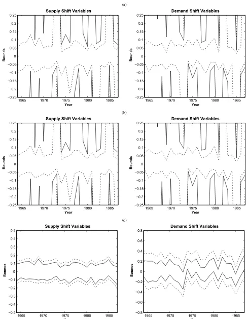
Figures 2 through 6 show estimates of the sharp bounds on the labor supply and demand shift variables for all sam-ples (Figure2), male samples (Figure3), female samples (Fig-ure4), high-school equivalents (Figure5), and college equiva-lents (Figure6). The solid lines represent the estimates of the
upper and lower bounds, the dotted lines represent the 10th and 90th bootstrap percentiles. In line with Lemmas1,2, and3, I as-sume the distributions ofεit andξit: (i) the distributions have a
zero median fori[Figure2(a)]; (ii) the distributions are sym-metric around zero fori[Figure2(b)]; and (iii) the distributions are time-invariant and normal distributions overi, where their means are zero and their variances are the middle of the mini-mum and maximini-mum estimates of the variances, as elaborated in Appendix F[Figures2(c),3,4,5, and6]. As Lemmas1and2 show, in cases (i) and (ii), only one side of the bound estimates is bounded. Some bound estimates in case (ii) are tighter than those in case (i). Specifically, in years when the observations whosepitis greater (smaller) thanpitare more than one-half of
all observations, the upper (lower) bound estimates onμand the lower (upper) bound estimates onνexist. When the proportion of these observations is large, there is a high possibility that the bound estimates in case (ii) are tighter than those in case (i). In case (iii), both bounds are estimated, and these bound estimates are significantly tighter than those in cases (i) and (ii). There-fore, imposing the assumption that the distributions are normal distributions has sufficient identification power to explain the shifts in the supply and demand curves. To compare the find-ings with those of previous studies, I principally use the bound estimates in case (iii) for interpretation.
The stylized facts regarding the between-group wage struc-ture changes are: (1) the male and female wage differentials were stable in the 1960s and 1970s, and decreased substan-tially in the 1980s and (2) the college wage premium rose in the 1960s, declined in the 1970s, and increased sharply in the 1980s (refer to Katz and Murphy1992; Murphy and Welch1992; Blau and Kahn1997,1999; and Katz and Autor1999).
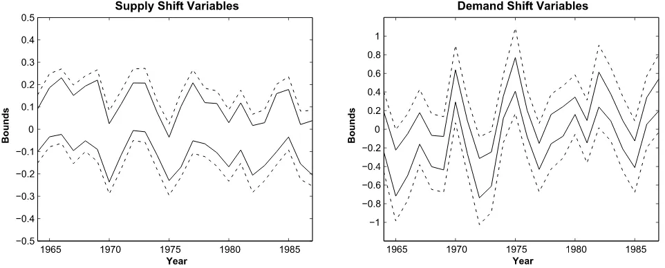
The male and female wage differentials(Figures3,4, and7): The supplies of male and female labor were stable. In the 1980s, the demand for male (female) labor was lower (higher) than in the 1960s. In the 1970s, the demand for male and female labor fluctuated.
Figure7shows the bound estimates of the difference between male and female labor shift variables. (The bound is explained in Appendix F.) The averages of the bound estimates in the 1960s, 1970s, and 1980s are shown by dashed lines. The rel-ative demand for male labor, as compared to that for female la-bor, has decreased, which caused the gender wage gap to shrink in the 1980s.
The college wage premium(Figures5,6, and8): The supplies of high-school and college equivalents were stable, whereas the latter slightly decreased in the 1980s. The demands for high-school and college equivalents fluctuated. In particular, the de-mand for college equivalents was lower in the 1970s than in other periods and increased sharply after 1977, while the de-mand for high-school equivalents decreased after 1980.
Figure 8 graphs the bound estimates of the difference be-tween shift variables of college and high-school equivalents. The relative demand for college equivalents, as compared to high-school equivalents, drifted downward during the 1970s. This trend reversed sharply in the 1980s, however. In contrast to the demand shifts, the relative supply of college equivalents, as compared to high-school equivalents, increased slightly in the 1970s and decreased in the 1980s. These shifts explain why the college wage premium rapidly rose from 1980, following a small decline in the 1970s.
(a)
(b)
(c)
Figure 2. (a) Estimates of the bounds on shift variables for all samples assuming the median of the disturbances is zero. (b) Estimates of the bounds on shift variables for all samples assuming the distributions of the disturbances are symmetric about zero. (c) Estimates of the bounds on shift variables for all samples assuming the distributions of the disturbances are normal. The solid lines are the estimates of the bounds and the dotted lines are the 10th and 90th bootstrap percentiles. [In (c), only 10th percentiles of the lower bounds and 90th percentiles of the upper bounds are shown.] In (a) and (b), the opposite sides of the bounded sides of the estimates (the solid lines) are not bounded (∞or−∞).
Figure 3. Estimates of the bounds on shift variables for males assuming the distributions of the disturbances are normal. The solid lines are the estimates of the bounds. The dotted lines are the 10th bootstrap percentiles of the lower bounds and the 90th bootstrap percentiles of the upper bounds.
Sixty-four groups of data are also classified into four cate-gories: male high-school equivalents, male college equivalents, female high-school equivalents, and female college equivalents. Using these categories, I estimate the supply and demand shift variables. The estimation results show that in the 1980s, mand for both male and female high-school equivalents de-creased; this demand, however, decreased faster for males than for females. The supply of male high-school equivalents in-creased in the 1980s, whereas the supply of female high-school equivalents decreased from the mid-1970s to the mid-1980s. This finding accounts for why male and female wage differen-tials decreased more rapidly for high-school equivalents than for college equivalents. (The estimation results are available from the author upon request.)
These estimation results are consistent with the findings of Katz and Murphy (1992), Murphy and Welch (1992), Blau and
Kahn (1997, 1999), and Katz and Autor (1999). In particu-lar, Katz and Murphy (1992) and Katz and Autor (1999) sug-gested that skill-biased technological change, shifts in product demand across industries, and rising international competition increased demand for educated labor in the 1970s and 1980s. Katz and Murphy (1992) illustrated the possibility that a de-crease in the growth rate of the supply of college graduates may help explain the increase in the college wage premium in the 1980s. By estimating sharp bounds on the supply and demand shift variables for gender and educational groups, this article provides evidence supporting their findings. To further study the causes of supply and demand shifts, the gender and educational groups can be divided into industry and occupa-tional groups. Utilizing this study’s approach, the within- and between-industry shifts of the supply and demand functions can be estimated.
Figure 4. Estimates of the bounds on shift variables for females assuming the distributions of the disturbances are normal. The solid lines are the estimates of the bounds. The dotted lines are the 10th bootstrap percentiles of the lower bounds and the 90th bootstrap percentiles of the upper bounds.
Figure 5. Estimates of the bounds on shift variables for high school equivalents assuming the distributions of the disturbances are normal. The solid lines are the estimates of the bounds. The dotted lines are the 10th bootstrap percentiles of the lower bounds and the 90th bootstrap percentiles of the upper bounds.
4. CONCLUSION
This article presents a nonparametric econometric model that identifies sharp bounds for the supply and demand shift vari-ables in a simultaneous equations model by only using ob-servations of the intersections of upward sloping supply and downward sloping demand curves. To clarify the causes of the changes in the wage differentials across gender and educational groups, labor supply and demand factors are estimated using panel data of wages and labor inputs. The estimation results show that (1) the relative demand for female labor, as compared to male labor, has increased in the 1980s and (2) the relative demand for college equivalents, as compared to high-school equivalents, slightly decreased in the 1970s and increased in the 1980s.
Since the assumption for identification is much less restric-tive than that of the existing parametric approach, the estimated bounds are large. Additional assumptions on disturbances nar-row the bounds. Two important research inquiries have yet to be considered: how to select assumptions on disturbances and the normalization point. These topics, however, are left for future study.
APPENDIX A: PROOF OF PROPOSITION1
Sincef is monotone increasing inp, for any real numberα, (q,p)∈
SE(α) ⇒ u> α, (q,p)∈NW(α) ⇒ u≤α.
Thus,
P((q,p)∈SE(α))≤P(u> α)≤1−P((q,p)∈NW(α)).
Figure 6. Estimates of the bounds on shift variables for college equivalents assuming the distributions of the disturbances are normal. The solid lines are the estimates of the bounds. The dotted lines are the 10th bootstrap percentiles of the lower bounds and the 90th bootstrap percentiles of the upper bounds.
Figure 7. Estimates of the bounds on the difference between male and female shift variables assuming the distributions of the disturbances are normal. The solid lines are the estimates of the bounds. The dashed lines are the averages of the bound estimates in the 1960s, 1970s, and 1980s.
These bounds are sharp since the empirical evidence and prior information are consistent with the hypothesisP((q,p)∈
SE(α))=P(u> α)and also with the hypothesis 1−P((q,p)∈
NW(α))=P(u> α). Hypothesis P((q,p)∈SE(α))=P(u> α) is consistent with the case in which all supply curves traversing the observations in NE(α) have enough gentle slopes for their u’s to be smaller than α, and all supply curves traversing the observations in SW(α) have enough steep slopes for theiru’s to be smaller thanα.The hypothe-sis 1−P((q,p)∈NW(α))=P(u> α) is consistent with the case in which all supply curves traversing the observations in NE(α) have enough steep slopes for their u’s to be greater than α, and all supply curves traversing the observations in SW(α) have enough gentle slopes for their u’s to be greater thanα.
SinceP(u> α)=1−Fu(α), for any real numberα,
P((q,p)∈NW(α))≤Fu(α)≤1−P((q,p)∈SE(α)).
These bounds are sharp.
Sincegis monotone decreasing inp, for any real numberα
(q,p)∈
NE(α) ⇒ v> α, (q,p)∈SW(α) ⇒ v≤α.
Thus
P((q,p)∈NE(α))≤P(v> α)≤1−P((q,p)∈SW(α)).
These bounds are sharp since empirical evidence and prior information are consistent with the hypothesis P((q,p)∈
NE(α))=P(v> α)and also with the hypothesis 1−P((q,p)∈
SW(α))=P(v> α). Hypothesis P((q,p)∈NE(α))=P(v>
Figure 8. Estimates of the bounds on the difference between shift variables of college and high-school equivalents assuming the distributions of the disturbances are normal. The solid lines are the estimates of the bounds. The dashed lines are the averages of the bound estimates in the 1960s, 1970s, and 1980s.
α)is consistent with the case in which all demand curves tra-versing the observations in SE(α) have enough gentle slopes for their v’s to be smaller than α, and all demand curves tra-versing the observations in NW(α) have enough steep slopes for theirv’s to be smaller thanα.The hypothesis 1−P((q,p)∈
SW(α))=P(v> α)is consistent with the case in which all de-mand curves traversing the observations in SE(α)have enough steep slopes for theirv’s to be greater than or equal toα, and all demand curves traversing the observations in NW(α)have enough gentle slopes for theirv’s to be greater thanα.
SinceP(v> α)=1−Fv(α), for any real numberα,
P((q,p)∈SW(α))≤Fv(α)≤1−P((q,p)∈NE(α)).
These bounds are sharp.
APPENDIX B: PROOF OF LEMMA1
Equations (3) and (5) imply that
u≤α1,
since
0.5≤P[(q,p)∈NW(α1)] ≤Fu(α1),
0.5≤Fu(u),
and
u=min{u|Fu(u)≥0.5}.
Equations (3) and (5) imply that
α2≤u,
since
0.5≤Fu(u)≤1−P[(q,p)∈SE(u)],
0.5≤1−P[(q,p)∈SE(α2)],
and
α2=inf
α|1−P[(q,p)∈SE(α)] ≥0.5.
Hence,
α2≤u≤α1.
This bound is sharp, since the bound in Equation (3) is sharp. That is, empirical evidence and prior information are consistent with the hypothesisu=α1and also with the hypothesisu=α2.
uis bounded on one side. For the sake of contradiction, sup-pose that α1= ∞ and α2= −∞. Since α1= ∞, by
Equa-tion (5), the set of {α|P[(q,p)∈NW(α)] ≥0.5} is empty. Therefore, for any α ∈R, P[(q,p)∈ NW(α)]<0.5. Thus,
P[p>p]<0.5. Since α2= −∞, by Equation (5), for any
α∈R,1−P[(q,p)∈SE(α)] ≥0.5.Thus,P[p>p] ≥0.5.This is a contradiction. Hence,uis bounded on one side.
uis never bounded on both sides. (The author thanks the ref-eree for providing the following proof.) Ifα2>−∞,there
ex-ists a∈(−∞, α2),such that 1−P[(q,p)∈SE(a)]<0.5
be-cause of the definition ofα2.Therefore, ifα2>−∞,then
0.5>1−P[(q,p)∈SE(a)] =1−P[q>q+a,p≤p] ≥1−P[p≤p] =P[p>p].
However, for anya,
P[(q,p)∈NW(a)] =P[q≤q+a,p>p] ≤P[p>p].
Hence, there does not exist a such that P[(q,p)∈NW(a)] ≥
0.5.
The set of {α|P[(q,p)∈NW(α)] ≥0.5}is empty. There-fore, by Equation (5),α1=inf∅ = ∞.
Ifα1<∞,P[(q,p)∈NW(α1)] ≥0.5.For anya,
1−P[(q,p)∈SE(a)] =1−P[q>q+a,p≤p] ≥1−P[p≤p] =P[p>p] ≥P[q≤q+α1,p>p] =P[(q,p)∈NW(α1)] ≥0.5.
Hence, α2= −∞. (The set of {α|1−P[(q,p)∈SE(α)] ≥
0.5}is not bounded below.) Therefore, ifα2>−∞,α1= ∞,
whereas ifα1<∞,α2= −∞.
Similarly,
β2≤v≤β1.
This bound is sharp.vis bounded on one side; however, it is never bounded on both sides.
APPENDIX C: PROOF OF LEMMA2
Define theγ quantile ofFuasmuγ. Equations (3) and (7) and
the definition ofmuγ imply that
muγ ≤α1(γ ),
since
γ≤P(q,p)∈NW(α1(γ ))≤Fu[α1(γ )],
γ≤Fu(muγ),
and
muγ =min{m|Fu(m)≥γ}.
Equations (3) and (7) and the definition ofmuγ imply that
α2(γ )≤muγ,
since
γ ≤Fu(muγ)≤1−P[(q,p)∈SE(m
u
γ)],
γ ≤1−P(q,p)∈SE(α2(γ )),
and
α2(γ )=infα|1−P[(q,p)∈SE(α)] ≥γ.
Hence,
α2(γ )≤muγ ≤α1(γ ). (C.1)
Similarly, for the(1−γ )quantile ofFu
α2(1−γ )≤mu1−γ ≤α1(1−γ ). (C.2)
Since the symmetry of the distribution ofuaroundu implies
muγ −u= −(mu1−γ−u), Equations (C.1) and (C.2) imply that
[α2(γ )+α2(1−γ )]/2≤u≤ [α1(γ )+α1(1−γ )]/2. (C.3)
Since the inequality in Equation (C.3) holds for anyγ∈ [0,1],
Let us show that these bounds are sharp. It suffices to show that for any sample size n, there exist the following two types of {ui}ni=1. Type (C-1) {ui}ni=1 satisfy the
condi-tions that (C-i){ui}ni=1realizeu=supγ∈[0,1][α2(γ )+α2(1−
γ )]/2, (C-ii) {ui}ni=1 are symmetrically distributed around u,
(C-iii) the supply curve corresponding toui traverses(qi,pi),
and (C-iv) all of the supply curves are upward sloping, i.e.,ui≥
qi forpi≤pandui≤qiforpi>p. Type (C-2){ui}ni=1satisfy
the conditions that (C-v){ui}ni=1realizeu=infγ∈(0,1)[α1(γ )+
α1(1−γ )]/2,(C-ii), (C-iii), and (C-iv).
Let us show that there exist{ui}ni=1of type (C-1). Defineq(i)
fori≤k1,as theith order statistics of{qj}whosep’s are greater
thanp; wherek1is the number of the observations withpbeing
greater thanp. Defineq(i) for i=k1+1,k1+2, . . . ,n as the
curves traversing the observations ofq(n−i)are vertical). Then,
it is possible to takeul(i) for k1+1≤i≤n/2,such thatuL−
Consequently, this distribution of ui, which is symmetric
aroundu and for which the corresponding supply curves are upward sloping, impliesu=supγ∈[0,1][α2(γ )+α2(1−γ )]/2.
Similarly, it is shown that there exist{ui}ni=1of type (C-2).
Therefore, in Equation (8) the bounds onuare sharp. The bounds onu in Lemma2 are tighter than or equal to those in Lemma1because supγ∈[0,1][α2(γ )+α2(1−γ )]/2≥
α2(0.5)=α2and infγ∈(0,1)[α1(γ )+α1(1−γ )]/2≤α1(0.5)=
α1.
u is bounded on one side becauseu is bounded on one side in Lemma1and the bounds on uin Lemma2are tighter than or equal to those in Lemma1.
Let us show that under Assumption1 the unbounded sides ofu in Lemma1are not bounded. Sinceuis bounded on one side in Lemma1, the opposite sides of the unbounded sides are bounded in Lemma1. These bounded sides are also bounded in Lemma 2because the bounded sides of uin Lemma 1 are also bounded in Lemma2. (This is because the bounds onuin Lemma2are tighter than or equal to those in Lemma1.) Since
uis never bounded on both sides in Lemma2, the opposite sides of these bounded sides are not bounded in Lemma2. Therefore, the unbounded sides in Lemma1are not bounded in Lemma2.
Similarly forv, it is proven that sup
γ∈[0,1]
[β2(γ )+β2(1−γ )]/2
≤v≤ inf
γ∈(0,1)[β1(γ )+β1(1−γ )]/2.
These bounds are sharp, as the empirical evidence and prior information are consistent with the hypothesis v =
supγ∈[0,1][β2(γ )+β2(1−γ )]/2 and also with the
hypothe-sisv=infγ∈(0,1)[β1(γ )+β1(1−γ )]/2. The bounds on vin
Lemma2 are tighter than or equal to those in Lemma1.vis bounded on one side; it is never bounded on both sides, how-ever. Under Assumption1the unbounded sides ofvin Lemma1 are not bounded. The proof is similar to that foruand is avail-able from the author upon request.
APPENDIX D: PROOF OF LEMMA3
AsFu(α)=Fu(α−u), Equation (3) implies that
P((q,p)∈NW(α))≤Fu(α−u)≤1−P((q,p)∈SE(α)).
SinceFuis known and strictly increases, by taking the inverse
ofFu
α−Fu−11−P((q,p)∈SE(α))
≤u≤α−F−u1P((q,p)∈NW(α)).
This holds for any real numberα;
sup
Let us show that this bound is sharp. It suffices to show that for any n there exist the following two types of {ui}ni=1.
Type (D-1) {ui}ni=1satisfy the conditions that (D-i){ui}ni=1
re-alizeu=supα{α−Fu−1[1−P((q,p)∈SE(α))]}, (D-ii){ui}ni=1
are distributed in quantiles ofFu, (D-iii) the supply curve
cor-responding to ui traverses(qi,pi), and (D-iv) all of the
sup-anduL are newly defined and different from those in
Appen-dix C.)
The first inequality holds because of the definition ofuL. Hence,
q(i)≤ul(i) for k1<i≤n. Thus, the supply curves traversing
ul(i) and the observations withq(i) fork1<i≤nhave positive
slopes. The positive slopes of the counterparts fori≤k1will be
shown later.
n.Therefore, the supply curves traversinguh(i)and the observa-tions withq(i)fork1≤i≤nhave positive slopes.
Similarly, asFv(β)=Fv(β−v)andFvis known and strictly
increases, Equation (4) implies that
sup
These bounds are sharp since the empirical evidence and prior information are consistent with the hypothesisP((q,p)∈
SE∗(α))=P(u> α)and also with the hypothesis 1−P((q,p)∈ cause of Assumption3,u> α foru’s that are associated with
(q,p)in NE∗(α)and SW∗(α).
SinceP(u> α)=1−Fu(α), for any real numberα,
P((q,p)∈NW∗(α))≤Fu(α)≤1−P((q,p)∈SE∗(α)).
These bounds are sharp.
Similarly,
beginning, the middle, and the end of the sample periods),
qit=qisandpit=pis(s=1,T/2,T). The interpretation of the
estimation results regarding the causes of gender and educa-tional wage differentials does not change. Estimation results are available from the author upon request.
(2)Group and category: The sample is divided into 64 groups distinguished by two sex categories, four education categories (8–11, 12, 13–15, and 16+years of schooling), and eight ex-perience categories (1–5, 6–10, 11–15, 16–20, 21–25, 26–30, 31–35, and 36–40 years).
High-school equivalents consist of those with 8–12 years of schooling (high-school graduates and high-school dropouts). College equivalents consist of those with 13–15 and 16+years of schooling (college graduates and those with some college).
(3) Variances of normal distributions in case (iii): Mini-mum variance is attained when the lengths of the estimated bounds of the shift variables in some years are zero and positive in other years. Since the length of the estimated bounds increases as the variance increases, the maximum vari-ance is attained when the length of the estimated bounds is longest. This longest length of the estimated bounds of the supply shift variables is the distance between the max-imum q-values of the observations where p >p and the minimum q-values of the observations where p ≤ p. The counterpart of the demand shift variables is the distance between the maximum q-values of the observations where
p≤p and the minimum q-values of the observations where
p>p.
(4)Bound estimates of the difference of shift variables be-tween groups: In Figure 7, the lower bound estimates of the difference between the male and female labor shift variables are identified by subtracting the female upper bound estimates from the male lower bound estimates. The upper bound esti-mates are calculated by subtracting the female lower bound timates from the male upper bound estimates. These bound es-timates are not sharp. The bound eses-timates of the difference between shift variables of college and high-school equivalents in Figure 8 are similarly derived.
ACKNOWLEDGMENTS
This is a revision of a chapter of my dissertation from North-western University. An earlier version of this article was enti-tled “Nonparametric Estimation of Supply and Demand Factors
with Applications to Labor and Macro Economics.” The author thanks two anonymous referees, an associate editor, the editor Arthur Lewbel, Joseph Altonji, Gadi Barlevy, Lawrence Chris-tiano, Jia-Young Fu, Roza Matzkin, Fumio Ohtake, Joon Y. Park, Christopher Taber, Elie Tamer, Emiko Usui, Randal Wat-son, Zhixiong Zeng, and especially Charles Manski for their helpful comments. The author thanks Lawrence Katz for send-ing his dataset. He also thanks participants at the seminars from the Econometric Society Summer Meeting, the European Meet-ing of the Econometric Society, the Annual Congress of the Eu-ropean Economic Association, the Midwest Macro Conference, the Far Eastern Econometric Society Conference, Northwestern University, Hitotsubashi University, Osaka University, the Uni-versity of Tokyo, Yokohama National UniUni-versity, the Institute of Statistical Research, and the Tokyo Center of Economic Re-search. A grant-in-aid for Scientific Research from JSPS and a research grant from the Japanese Bankers Association are also greatly appreciated.
[Received March 2008. Revised October 2009.]
REFERENCES
Blau, F. D., and Kahn, L. M. (1997), “Swimming Upstream: Trends in the Gen-der Wage Differential in the 1980s,”Journal of Labor Economics, 15, 1–42. [177,179]
(1999), “Institutions and Laws in the Labor Market,” inHandbook of Labor Economics, Vol. 3A, eds. O. Ashenfelter and D. Card, Amsterdam, The Netherlands: Elsevier. [177,179]
Blundell, R., Gosling, A., Ichimura, H., and Meghir, C. (2007), “Changes in the Distribution of Male and Female Wages Accounting for Employment Composition Using Bounds,”Econometrica, 75, 323–363. [175]
Brown, D. J., and Matzkin, R. L. (1998), “Estimation of Nonparametric Func-tions in Simultaneous EquaFunc-tions Models, With an Application to Consumer Demand,” CFDP 1175, Cowles Foundation for Research in Economics, Yale University. [175]
Ekeland, I., Heckman, J. J., and Nesheim, L. (2004), “Identification and Esti-mation of Hedonic Models,”Journal of Political Economy, 112, 60–109. [175]
Katz, L. F., and Autor, D. H. (1999), “Changes in the Wage Structure and Earn-ings Inequality,” inHandbook of Labor Economics, Vol. 3A, eds. O. Ashen-felter and D. Card, Amsterdam, The Netherlands: Elsevier. [177,179] Katz, L. F., and Murphy, K. M. (1992), “Changes in Relative Wages, 1963–
1987: Supply and Demand Factors,”Quarterly Journal of Economics, 107, 35–78. [174,177,179]
Lewbel, A. (2008), “Using Heteroskedasticity to Identify and Estimate Mis-measured and Endogenous Regressor Models,” Working Paper in Eco-nomics 587, Boston College, Dept. of EcoEco-nomics. [175]
Manski, C. F. (1994), “The Selection Problem,” inAdvances in Econometrics:
Sixth World Congress, Vol. 1, ed. C. Sims, Cambridge, U.K.: Cambridge University Press. [175]
(1997), “Monotone Treatment Response,”Econometrica, 65, 1311– 1334. [175,176]
Manski, C. F., and Pepper, J. (2000), “Monotone Instrumental Variables: With an Application to the Returns to Schooling,”Econometrica, 68, 997–1010. [175]
Matzkin, R. L. (2007), “Nonparametric Identification,” inHandbook of Econo-metrics, Vol. 6B, eds. J. J. Heckman and E. E. Leamer, Amsterdam, The Netherlands: Elsevier. [175]
(2008), “Identification in Nonparametric Simultaneous Equations Models,”Econometrica, 76, 945–978. [175]
Murphy, K. M., and Welch, F. (1992), “The Structure of Wages,”Quarterly Journal of Economics, 107, 285–326. [174,177,179]
Murphy, K. M., Riddell, W. C., and Romer, P. M. (1998), “Wages, Skills, and Technology in the United States and Canada,” inGeneral Purpose Tech-nologies and Economic Growth, ed. E. Helpman, Cambridge: MIT Press. [177]
Rigobon, R. (2003), “Identification Through Heteroskedasticity,” Review of Economics and Statistics, 85, 777–792. [175]