Full Terms & Conditions of access and use can be found at
http://www.tandfonline.com/action/journalInformation?journalCode=cbie20
Download by: [Universitas Maritim Raja Ali Haji] Date: 18 January 2016, At: 19:25
Bulletin of Indonesian Economic Studies
ISSN: 0007-4918 (Print) 1472-7234 (Online) Journal homepage: http://www.tandfonline.com/loi/cbie20
Poverty in Indonesia 1984–2002: the impact of
growth and changes in inequality
Riyana Miranti
To cite this article: Riyana Miranti (2010) Poverty in Indonesia 1984–2002: the impact of growth and changes in inequality, Bulletin of Indonesian Economic Studies, 46:1, 79-97, DOI: 10.1080/00074911003642252
To link to this article: http://dx.doi.org/10.1080/00074911003642252
Published online: 17 Mar 2010.
Submit your article to this journal
Article views: 407
View related articles
ISSN 0007-4918 print/ISSN 1472-7234 online/10/010079-19 © 2010 Indonesia Project ANU DOI: 10.1080/00074911003642252
POVERTY IN INDONESIA 1984–2002:
THE IMPACT OF GROWTH AND CHANGES IN INEQUALITY
Riyana Miranti*
University of Canberra
This paper examines the growth elasticity of poverty across three development epi-sodes in Indonesia between 1984 and 2002, after controlling for inequality. It relies on estimation of panel data from the National Socio-Economic Survey conducted by the central statistics agency. Contrary to expectations, the growth elasticity of poverty was virtually indistinguishable across the three development episodes – a period of far-reaching policy liberalisation (1984–90); a second period of slower liberalisation (1990–96); and the period of recovery from the Asian fi nancial crisis
(1999–2002). Growth was pro-poor in all three periods, while the impact of growth on poverty was either augmented or offset by changes in inequality, depending on the period. Only during the fi rst liberalisation period did a reduction in inequality
serve to augment the impact of growth on poverty.
INTRODUCTION
The incidence of poverty in Indonesia fell from 29.5% in 1984 to 18.2% in 2002,
although the decline was interrupted for a few years by the fi nancial crisis of the
late 1990s. The fi rst objective of this paper is to examine the impact of economic
growth on poverty, with a special focus on differences during periods of policy
liberalisation and crisis recovery. It does not attempt, however, to reach defi nitive
conclusions about why the impact differed across time.
Most previous studies measuring the impact of economic growth on poverty, including those on Indonesia, have used a short time-frame and have not exam-ined differences in impact across different time periods (for example, Bidani and Ravallion 1993; Balisacan, Pernia and Asra 2003; Miranti and Resosudarmo 2005). This may be due to data limitations, as a longer time series is necessary for an extended analysis. Friedman (2005) did extend his focus to a 15-year period (1984–99), but did not decompose this longer time-frame into shorter develop-ment episodes. The analysis in this paper is undertaken for the years 1984–2002, and the period is divided into three development episodes, 1984–90, 1990–96 and 1999–2002. The purpose of considering these three sub-periods separately is to shed some empirical light on the view that differing government policies across these sub-periods had different impacts on poverty.
* riyana.miranti@natsem.canberra.edu.au. I am grateful to Chris Manning, Hal Hill, Budy
Resosudarmo, Ross McLeod and two anonymous referees for their advice on previous drafts. Those who gave advice bear no responsibility for any errors or defi ciencies in the fi nal version.
If the distribution of income is constant, economic growth must reduce pov-erty. If income distribution becomes more equal, this tends to reduce poverty, and conversely. The second objective of this paper is therefore to determine the extent to which poverty reduction was simply the consequence of growth, and to what extent this effect was augmented or offset by changes in inequality.
DEFINITIONS AND DATA Poverty
To calculate the growth elasticity of poverty we focus on the head-count ratio or incidence of poverty – that is, the proportion of poor people in the total popu-lation. People are categorised as poor when their consumption is below a cer-tain threshold, referred to as the poverty line. Henceforth, ‘poverty’ as used in this paper refers to poverty as measured by the poverty head-count ratio. This paper applies the poverty line methodology currently used by the central
statis-tics agency (BPS), the offi cial institution publishing poverty data for Indonesia
(BPS 2003). BPS adopts the ‘basic needs’ approach, defi ning the poverty line as
the cost of consuming 2,100 calories per person per day, plus a pro-rata allowance for non-food requirements. This approach differs from the analysis of Friedman (2005), who applied the methodology of Bidani and Ravallion (1993) and Raval-lion (1994) in constructing his poverty lines, and calculated the cost of non-food needs in terms of the cost of foregone food items.
BPS claims that its current methodology is more comparable across regions and consistent across time than previous methods. It has used this method
since it revised the 1996 offi cial poverty fi gure. Three signifi cant methodological
improvements have been introduced (BPS 2003). First, the measure includes more commodities as basic needs. Second, consistency across time has been improved by applying the 1999 shares of total consumption (proxied by expenditure) for each of 52 products. The expenditure share of each product in the bundle differs across provinces but is similar over time. Third, comparability across provinces has been improved by indexing the price level in each province to the price level in Jakarta, such that the cost of the ‘basic needs’ basket of goods is comparable for the reference populations in all provinces. Thus, regional disparities in consumption arise only because of differences in consumption patterns and prices, and not
because of differences in income levels.1 The methodology is considered dynamic
in the sense that different consumption tastes and patterns among provinces are taken into account.
As a preliminary step, this paper uses the improved BPS methodology to
re-calculate poverty incidence between 1984 and 1996, the year the offi cial poverty
fi gure was revised.2 Applying the new methodology results in poverty levels
for the period 1984–93 that are different from those offi cially published by BPS.
Table 1 shows the offi cial poverty series and the re-calculated poverty levels used
in this paper.
1 However, the BPS poverty line has some shortcomings, especially in relation to regional price differences, which are calculated and discussed in Nashihin (2007).
2 For a full description of the process, see Miranti (2007).
The poverty level is calculated using a panel of seven consecutive
cross-sectional National Socio-Economic Surveys (SurveiSosial Ekonomi Nasional, or
Susenas) undertaken by BPS from 1984 to 2002, covering 26 provinces.3 While
the core Susenas survey is conducted annually, a Susenas module covering con-sumption is published every three years. Since 1981, the concon-sumption module sample has covered approximately 65,000 households. Quantity and value data are collected on more than 300 items for representative households in each prov-ince. The present study covers the period 1984–2002, using the 1984, 1987, 1990, 1993, 1996, 1999 and 2002 consumption modules (that is, seven waves). Use of provincial-level data provides far more observations of growth and inequality than would relying on national data, and hence results in more reliable econo-metric estimates.
Growth
The term ‘economic growth’ is most commonly understood to refer to a change in the level of gross domestic product (GDP), a measure reported in the national accounts, and its regional counterpart, gross regional domestic product (GRDP). However, changes in the welfare of a country’s people may also be represented by other measures. Aggregate household income, estimated from household sur-veys, is one of these.
Deaton (2001: 127) has criticised attempts to use growth data from the national accounts to study the relationship between growth and poverty. He argues that this growth measure ‘has at best a weak relationship with poverty’, since the national accounts data and the household surveys used for calculating poverty
3 For consistency, four new provinces – Bangka Belitung, Banten, Gorontalo and North Maluku – which fi rst appeared in the 2002 Susenas as a result of province fragmentation
– have been re-combined with the provinces they were separated from, in order to match the former provinces of South Sumatra, West Java, North Sulawesi and Maluku.
TABLE 1 Poverty, 1984–2002
(% of population)
Offi cial BPS Poverty Series New Poverty Seriesa
1984 21.7 29.5
1987 17.4 25.7
1990 15.1 23.4
1993 13.7 20.6
1996 11.3
1996 revised (see text) 17.6 17.6
1999 23.4 23.4
2002 18.2 18.2
a Recalculated by the author for 1984, 1987, 1990 and 1993, using the 2003 poverty line methodology of the central statistics agency (BPS).
Source: BPS, National Socio-Economic Survey (Susenas), various years.
levels measure different things. There are marked discrepancies in both direction and rate of change between the two types of growth data (table 2). It can therefore be argued that using an income proxy from the national accounts in conjunction with household survey poverty data introduces new errors, in addition to those found in the national accounts (Ravallion and Chen 1997: 363). The two types of errors do not cancel each other out (Ravallion 2003). We would expect the same problem to occur if an income proxy from the regional accounts were used.
Adams (2004) found that the growth elasticity of poverty is sensitive to the meas-ure of income used. Most traditional empirical estimations of the growth elasticity of poverty use mean consumption expenditure from household surveys as a proxy
for income (Adams 2004). It has been argued that this proxy is a better refl ection of
welfare than is income calculated from the same source (Ravallion 1995), because it gives a more accurate indication of ‘life-cycle’ or permanent (that is, long-term) income (Balisacan, Pernia and Asra 2003: 332). Moreover, the data collected on con-sumption are more accurate than the income data, given that people may have rea-sons to hide some of their income (Ravallion 2001) and that measured consumption patterns are less variable than measured income patterns (Deaton 1997).
This study uses mean consumption from the household surveys as a proxy for income, and uses change in this variable as a proxy for economic growth. It uses the province as the spatial unit for calculating income and changes in income, and calculates monthly mean household consumption expenditure per capita for each
province in each Susenas consumption module period. Thus, ‘growth’ is defi ned
in this study as the percentage change in provincial monthly mean household consumption expenditure per capita (for simplicity, we refer to this below as ‘con-sumption expenditure per capita’). The term ‘growth elasticity of poverty’ refers to the percentage reduction in poverty given a 1% increase in mean consumption expenditure per capita (rather than given a 1% change in GDP or GRDP).
In this paper, mean consumption expenditure per capita is calculated in real terms, to allow comparison across time. Real mean consumption expenditure per
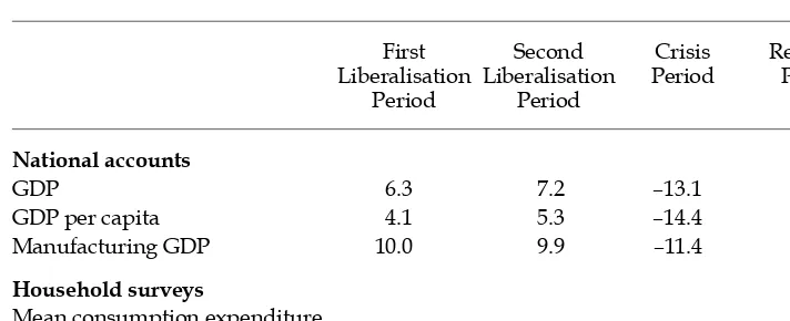
TABLE 2 Growth Rates by Growth Measure and Development Episode, 1984–2002
(% p.a)
Source: BPS, Susenas and national accounts, various years; CEIC Asia Database, various years. Data on mean consumption expenditure per capita for the crisis period are from Suryahadi, Sumarto and Pritchett (2003).
capita is calculated by defl ating mean consumption to 1984 prices. The defl ator
used is the implicit defl ator of the weighted average of the urban and rural
pov-erty lines, following Friedman (2001), Tarp et al. (2002) and Grimm and Gunther
(2006). The poverty line has been chosen as the defl ator in preference to the
con-sumer price index (CPI), because it gives a better representation of the spending patterns of the poor (Adams 2004). Food items comprise only 40% of the CPI, but they represent more than 70% of the items used to calculate the poverty line (BPS 2003). A further consideration is that the CPI is calculated only for 44 urban areas in Indonesia, and does not cover rural areas, even though price movements in
urban and rural areas may differ. Use of the CPI as the defl ator could therefore
result in biased estimates of real consumption.
DEVELOPMENT EPISODES
Between the 1970s and 2002, Indonesia experienced several distinct episodes of development, including the oil boom from 1972 to around 1981; the rice boom of 1978–83; a period of wide-ranging liberalisation throughout the mid- to late 1980s (Woo, Glassburner and Nasution 1994; Hill 2000); a second period of more cautious liberalisation (Hill 1997) – and some back-sliding on reform – during the
fi rst half of the 1990s; the fi nancial and economic crisis of 1997–98; and, fi nally,
recovery after the crisis, beginning in 1999. There is no clear consensus on when either of the two liberalisation periods started. One strand of the literature refers mainly to microeconomic reform – especially trade liberalisation – commencing in 1986 (Woo, Glassburner and Nasution 1994: 115) or 1987 (Hill 2000: 17), fol-lowing a sharp decline in world oil prices in 1986. Several liberalisation packages were introduced in 1986 to ease import and export procedures. They included
a duty exemption and drawback scheme that allowed export-oriented fi rms to
purchase imported inputs at international prices – the initial step towards an export-promoting path of industrialisation. But in addition to trade
liberalisa-tion there had been some earlier fi scal reforms (such as tax reforms in 1983 and
1985) and exchange rate reforms (a devaluation in 1983). Soesastro (2006)
dis-cusses these, and identifi es liberalisation as commencing in 1982. Aswicahyono
and Feridhanusetyawan (2004: 13) too have argued that microeconomic reform began in the period 1982–85, although they note that this reform was slower and
less effective than the liberalisation of the mid-1980s.4
The delineation of periods for analysis in this paper is therefore to some extent arbitrary, and has been driven partly by the availability of data at three-year inter-vals from the Susenas consumption module. The timing of the latter made 1984 a convenient starting point for the analysis, and 1984–90 and 1990–96 appropriate
time-spans for the fi rst and second liberalisation periods, while 1999–2002
realis-tically refl ects Indonesia’s crisis recovery period. Data for 1990, the transitional
year linking the fi rst and the second liberalisation periods, is included in both.
The following section discusses each of the development episodes. In explain-ing economic growth durexplain-ing each of the development episodes, two sources of
4 While trade liberalisation would have had a predictable impact on poverty, the impact of other kinds of reform on poverty is less clear.
growth data are discussed: the national accounts and the household surveys. Growth data from the latter source are then used in the estimation below.
The fi rst liberalisation period (1984–90)
During the fi rst liberalisation period, GDP grew by 6.3% annually. Manufacturing
GDP expanded by 10% p.a. (table 2) – almost twice the rate of GDP in
agricul-ture (5.1%; fi gure not shown). Per capita GDP growth was 4.1%, while per capita
expenditure consumption based on household survey data grew more slowly, at 1.1%. The difference in the rate of change between the national accounts (GDP)
data and the household survey data is the result of differences in the defi nition
and coverage of GDP and household consumption per capita.
This fi rst liberalisation period can be called one of transformation, in which
Indonesia experienced rapid industrialisation. There was initially a movement
away from heavy reliance on oil and gas exports and towards a more diversifi ed
economy based on a strongly export-oriented manufacturing sector. This was fol-lowed by a transformation of the structure of employment, away from the pri-mary sector and towards manufacturing and services.
Reform in the banking sector began in 1983, when the government removed ceilings on time deposit rates at state banks and lending controls at all banks. This was followed by a further banking deregulation package in 1988, which removed restrictions on the expansion of bank branch networks and the establishment of new banks, except in the case of purely foreign-owned banks (McLeod 1993; Aswicahyono and Feridhanusetyawan 2004). From March 1985 through May 1990, a number of other deregulation packages were launched to liberalise the economy, and especially to promote non-oil exports. The new policies included reform of export incentives and administrative improvements to simplify
proce-dures by reducing the number of licences required to export goods.5 As a result of
the trade reform and deregulation, tariffs and non-tariff barriers (NTBs) declined
signifi cantly (Fane 1996; Hill 2000; Aswicahyono and Feridhanusetyawan 2004).
Signifi cant growth in exports, structural transformation and poverty reduction
took place during this fi rst period (Hill 2000).
The sectoral transformation away from agriculture and towards manufacturing and services was mirrored in employment during the mid-1980s, with an expan-sion of jobs in footloose labour-intensive manufacturing sectors such as cloth-ing, woven fabrics, footwear, electronics, furniture, yarn, toys and sporting goods and glass and glassware (Hill 2000). Previous researchers (Hill 2000; Temple 2003) have argued that Indonesia’s growth during the 1980s was not only rapid but particularly favourable to the poor, because trade liberalisation policy meant that Indonesia could make better use of one of its abundant resources – low-skilled labour. This was readily available in large quantities in agriculture, and could be drawn out of that sector into more modern activities in manufacturing, construc-tion and other services, where its productivity would be higher and hence it could earn higher incomes. Thus policies at the time were consistent with the reality that the most straightforward way to reduce poverty is to increase the demand for
5 Hill (2000) points out that the strongest trade reform took place in the 1986–89 period, when protection was reduced progressively.
labour supplied by the poor. Restructuring the economy in line with comparative advantage through trade liberalisation was an obvious way to do this.
It has been argued that growth of the labour-intensive manufacturing sector, and of the economy as a whole, reduces poverty. For example, Manning (1998:
ch. 5) and Osmani (2004) have argued that declining poverty during the fi rst
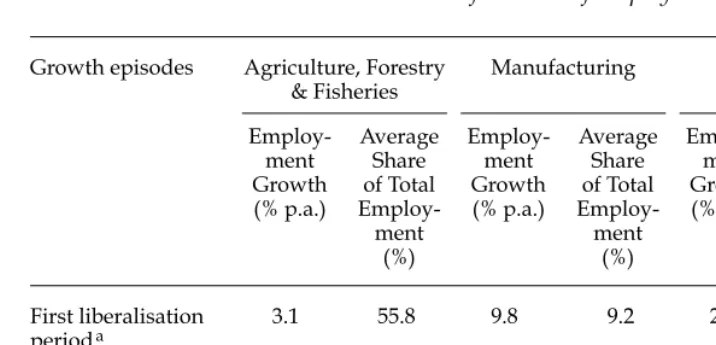
lib-eralisation period resulted mainly from the employment expansion created by economic growth, facilitated by slow growth in real wages. Table 3 illustrates this structural transformation of employment. The proportion of jobs in the
agricul-ture, forestry and fi sheries sector declined, while the share in manufacturing and
the services sector increased.
Average annual growth of employment in agriculture, forestry and fi
sher-ies during the fi rst liberalisation period was 3.1%, whereas in the
manufactur-ing sector it was more than three times as rapid, at 9.8%. Large quantities of labour were indeed drawn out of agriculture into more modern activities in manufacturing and services. During this period, the proportion of employed
persons working in agriculture, forestry and fi sheries was around 55.8% on
average, while 9.2% of employment was in the manufacturing sector and 30.5% in services.
The second liberalisation period (1990–96)
During the period 1990–96, GDP and GDP per capita grew even more rapidly, by 7.2% and 5.3% annually, while manufacturing output continued to grow at 9.9% (table 2). Mean consumption expenditure per capita grew slightly more rapidly
than in the fi rst liberalisation period, by 1.3% annually. Although the magnitude
of the two per capita growth rates differs, both measures increased during the
TABLE 3 Structural Transformation of Employment
Growth episodes Agriculture, Forestry & Fisheries
Recovery period 1.9 44.2 1.7 13.1 0.8 38.1
a Owing to data limitations, the fi rst liberalisation period starts at 1987 for agriculture, forestry and fi sheries and for manufacturing, and at 1989 for services, instead of at 1984. Data on employment in
other sectors (mining and quarrying; electricity, gas and water; and construction) are not shown in this table.
Source: CEIC Asia Database.
second liberalisation period. Liberalisation through deregulation policies weak-ened, however (Hill 1997). Aswicahyono and Feridhanusetyawan (2004) have labelled the (slightly different) period 1992–97 as one of ‘deregulation fatigue’. Reforms were slower and less comprehensive, and there was some return to more interventionist policy (Fane 1996). For example, a new monopoly on clove trading was introduced in 1991, as were new restrictions on inter-island trade in oranges from West Kalimantan in 1991; the tariff surcharge on imports of propylene and ethylene was increased in 1993. The government also established a ‘national’ car project involving Kia Motors of South Korea and the Indonesian car maker Timor Putra Nasional, under which Timor was exempted from paying luxury taxes (Fane 1996; Aswicahyono and Feridhanusetyawan 2004).
During the second liberalisation period, and especially between 1993 and 1996, there was a decline in the rate of job creation, particularly in manufacturing and agriculture, probably indicating that the previous labour surplus had begun to be exhausted. Employment growth in the manufacturing sector was slower
dur-ing the second liberalisation period, at 5.8%, than it had been in the fi rst, while
employment in the agricultural sector contracted by 1.9% per year (table 3). Do such data imply that growth was less pro-poor during this second liberali-sation period? In fact, poverty fell by nearly six percentage points in these years, from 23.4% in 1990 to 17.6% in 1996 – a slightly larger relative decline than in
the fi rst period (table 1). The faster rate of poverty decline was probably due to
increases in real wages in all sectors, including construction, textiles and govern-ment administration (Manning 1998: ch. 5; Feridhanusetyawan 2002), as the rapid
growth of manufactured exports fi nally began to have an impact on the general
price of unskilled labour. Real wages in the manufacturing sector grew by 33% between 1990 and 1996 – an annual growth rate of around 5%. On the other hand, as we will see below, inequality worsened during this period, with the Gini
coef-fi cient increasing noticeably, from 0.321 in 1990 to 0.355 in 1996. This seems to
indicate that as trade liberalisation progressed, its impact was less heavily con-centrated on the poor.
The crisis period (1997–98)
The Asian fi nancial crisis hit Indonesia in 1997. A political crisis followed that
culminated in Soeharto’s resignation from the presidency in 1998. The economy fell into turmoil, with GDP contracting by more than 13% (and GDP per capita by more than 14%) in 1998 (table 2). Mean consumption expenditure per capita also fell, by 17% (Suryahadi, Sumarto and Pritchett 2003).
It was decided not to include the period 1997–98 in the present analysis, because
the growth fi gure for the period as a whole masks enormous underlying
volatil-ity: the GDP growth rate fell from 4.7% in 1997 to –13.1% in 1998, before bouncing back to 0.8% in 1999. Under such circumstances, and recalling that the Susenas consumption module data are produced only every third year, it would be very
diffi cult to draw any meaningful interpretation of the overall change in the
pov-erty level during this period of turmoil.
The recovery period (1999–2002)
Following the crisis there was little by way of the kinds of policy reform that had been seen during the 1980s and early 1990s. Indeed, policy in the labour market
area – which is of crucial importance to poverty – began to become much more interventionist. The economy rebounded, with GDP growing at an average rate of 4% per annum, and per capita GDP at 2.7% per annum (table 2), though this growth was much slower than that in the two periods of liberalisation. How-ever, mean per capita consumption expenditure grew markedly in the recovery
period, at 3.3% p.a. This growth was more rapid than that in the fi rst and second
liberalisation periods, and suggests that, coming from a very low base during the crisis, consumption was quick to recover relative to other sectors. Miranti (2007: 77–8) shows that this recovery of mean consumption expenditure was
robust to the choice of defl ator.
The manufacturing sector recovered slowly to grow by only 4.2% per year during this period (table 2), less than half the rate during the two liberalisation phases. Despite the severe economic contraction during the crisis, unemployment had remained lower than expected (Feridhanusetyawan 2002). Instead, there was a shift of main occupation, with displaced workers moving from shrinking sec-tors to other secsec-tors – especially agriculture and the informal sector. In contrast with the two liberalisation periods, employment growth of 1.9% in agriculture,
forestry and fi sheries during the recovery phase, while slow, was slightly more
rapid than growth of employment in manufacturing, where jobs expanded at just 1.7% annually; services employment grew by only 0.8% during this period
(table 3). This adjustment refl ected the fl exibility of the labour market (Manning
2000; Feridhanusetyawan 2002).
Nevertheless, poverty fell by 5.2 percentage points in this recovery period, from 23.4% in 1999 to 18.2% in 2002, a level only slightly higher than that in 1996 (17.6%) (table 1). Suryahadi and Sumarto (2001) categorised people with per capita consumption below the poverty line immediately after the crisis as either
chronic or transient poor. The fi rst category refers to those likely to remain poor
in the future, and the second to those likely to increase their consumption suffi
-ciently to elevate themselves above the poverty line in the future. Suryahadi and
Sumarto found that the head-count ratio of transient poor increased from 12.4%
of the population in 1996 to 17.9% in 1999, whereas the head-count ratio of the
chronic poor increased by almost a factor of three, from 3.2% to 9.5%, during the same period. This shows that rising numbers of chronic poor contributed most to the increase in poverty, such that their share of the total rose from 20% to
35%. The fact that poverty declined during the recovery period may refl ect the
impact of renewed GDP growth in raising the consumption of those in transient poverty. Thus it is not surprising that inequality worsened during this period, because the recovery may have had less impact on the chronic poor than on other groups.
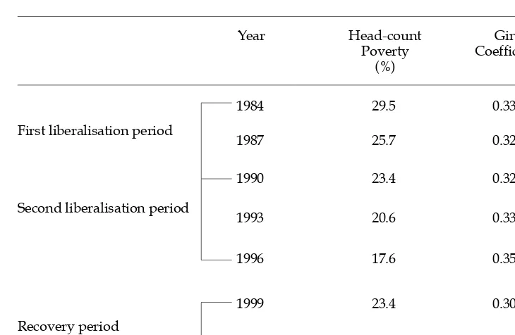
Changes in poverty and inequality
Table 4 shows the trends in poverty and in inequality (as indicated by the Gini
coeffi cient) during the three periods under consideration. During the fi rst
liberalisation period, poverty fell by about six percentage points (from 29.5% in 1984 to 23.4% in 1990), while inequality declined very slightly from 0.330 to 0.321. Poverty again fell by almost six percentage points – a larger relative decline – dur-ing the second liberalisation period, even though inequality increased noticeably, to 0.355 in 1996.
These changes were reversed during the crisis, but the recovery period saw poverty fall back to 18.2%, only a little higher than its level in 1996, while inequal-ity returned to around its 1984 level (table 4).
We turn now to estimate the extent to which changes in poverty can be attrib-uted to economic growth, on the one hand, and changing inequality on the other. The following section provides the empirical methodology for this estimation.
EMPIRICAL METHODOLOGY AND APPROACH
An absolute poverty measure will be a strictly decreasing function of an increase
of mean consumption (growth), given a fi xed poverty line and fi xed income
dis-tribution (or given that the consumption of each individual changes in the same proportion) (Ravallion 1995). This means that when income distribution is held constant, a positive change in mean consumption expenditure per capita (growth) will reduce poverty. This assumption of unchanging income distribution has been made in various studies that measure the impact of economic growth on poverty, including Datt and Ravallion (1992); Kakwani (1993); and Bourguignon (2003).
Thus the growth elasticity of poverty (GEP) is defi ned as the percentage reduction
in poverty given a 1% increase in consumption expenditure per capita, with other factors held constant.
In reality, however, income distribution, or the level of inequality, is also likely to vary over time. In this paper, the degree of inequality of the income
distribution is measured by the Gini coeffi cient, which has a value between
zero and one. A value of zero means perfect equality, such that everyone in the
TABLE 4 Poverty and Inequality 1984–2002
Year Head-count Poverty
(%)
Gini Coeffi cient
1984 29.5 0.330
First liberalisation period
1987 25.7 0.322
1990 23.4 0.321
Second liberalisation period
1993 20.6 0.335
1996 17.6 0.355
1999 23.4 0.308
Recovery period
2002 18.2 0.329
Source: BPS, Susenas, various years.
population has the same level of income. A value of one indicates perfect ine-quality, where one person accounts for all income. More generally, the smaller
the Gini coeffi cient, the more equal the distribution of income. An increase in
the Gini coeffi cient is likely to contribute positively to absolute poverty, other
things being equal. The inequality elasticity of poverty (IEP) is defi ned as the
percentage change in poverty given a 1% increase in the Gini coeffi cient, with
other factors held constant.
To estimate the growth and inequality elasticities of poverty, I follow a basic model suggested by Ravallion and Chen (1997):
lnPi t, lnMEANi t, lnGINIi t, e td
MEANi t, is mean consumption expenditure per capita (Rp/month, 1984 prices)
for province i at time t, as a proxy for income;
GINIi t, is the Gini coeffi cient for province i at time t, as a proxy for inequality.
t is the year index (t = 1984, 1987, 1990, 1993, 1996, 1999, 2002);
dt are the year dummies for the years when the Susenaswas conducted:
d87=1 if t = 1987, and 0 otherwise;
The base period is 1984.
δi is the province fi xed effect (unobserved heterogeneity).
εi t, is a white-noise error term that includes errors in the poverty measure.
As equation (1) is in logarithmic format for both dependent and independent
variables, the coeffi cient of lnMEAN refers to a 1% change in monthly mean
con-sumption per capita (as a proxy for income) and the coeffi cient of lnGINI refers to
a 1% change in inequality.
While Ravallion and Chen (1997) and Adams (2004) use fi rst differences
esti-mation, this paper uses fi xed effects, for the following reasons. First, fi xed-effects
estimation allows the use of all the information available, even though these are unbalanced panel data. They are unbalanced because there are several missing observations for poverty in 1990 in nine provinces (BPS did not publish the data for those provinces in that year), and because of the absence of consumption
data for Aceh, Maluku and Papua in 2002 (when a Susenasmodule could not be
undertaken in these provinces because of signifi cant social and political unrest).
Second, the fi xed-effects approach is more effi cient than the fi rst-differences
approach, because in any province random errors are usually assumed to be serially independent – that is, not serially correlated with each other across time periods (Wooldridge 2003).
Equation 1 assumes that the impact of growth on poverty is similar across periods, but responds to the possibility of omitted variable bias by incorporat-ing province and year dummies. The latter also capture, in general, the impact of
macroeconomic conditions in each Susenas consumption module period.
Com-parison of the coeffi cients of the year dummies with that for the base period of 1984
will indicate whether poverty was higher on average (if there is a signifi cant
posi-tive sign) or lower (if there is a signifi cant negative sign) than for the base period,
after the analysis has controlled for changes in consumption and in inequality. However, we also aim to discover whether there are differences in the growth and inequality elasticities of poverty across development episodes. Equation 2 therefore incorporates a set of interaction terms intended to determine whether the impact of growth and inequality on poverty differs across development episodes. The six year dummies are still included to avoid omitted variable bias and to capture, in general, the impact of macroeconomic conditions in each Susenas con-sumption module period. In addition, there are interactions between the second
liberalisation period (EPISODE2) and the recovery period (EPISODE3) with the
growth variable (lnMEAN). Similarly, in calculating the IEP across development
episodes, there are interactions between the Gini coeffi cient variable (lnGINI) and
both the second liberalisation period (EPISODE2) and the recovery period (
EPI-SODE3). The base period is the fi rst liberalisation period, 1984–90.
Thus we now have:
The reference development episode is 1984–90 (the fi rst liberalisation period).
To test the structural stability of the regression model (that is, to check whether there is a structural change in the overall relationship between growth and
pov-erty and between inequality and povpov-erty), I performed an F-test of joint signifi
-cance of the interaction terms.
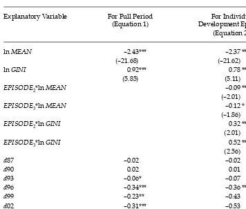
EMPIRICAL RESULTS Full period
We begin by assuming that the relationships between growth and poverty and inequality and poverty remained unchanged throughout the whole period. The middle column of table 5 shows that, after we had controlled for
inequal-ity, the GEP (lnMEAN) was –2.43 during the period 1984–2002. This means that
a 10% increase in consumption per capita reduced poverty proportionately by 24.3%. (By way of illustration, suppose that a particular province had a real mean
6 The dummies for the development episodes are used to capture the macroeconomic con-ditions during the specifi c development episodes.
consumption level of Rp 100,000 per month and a head-count poverty ratio of 20%. At a later time, when consumption had increased by 10% to Rp 110,000, pov-erty would have decreased by 24.3% of 20%, to 15.1%, other things being equal.)
The IEP (lnGINI) was 0.92, meaning that a 10% increase in inequality (as
meas-ured by the Gini coeffi cient) increased poverty proportionately by 9.2%.
The GEP in table 5 is similar to that found by Friedman (2005) for Indonesia over the period 1984–99. It is also comparable with that found in studies of other countries that also used the head-count poverty ratio measure as the dependent variable. For Bangladesh, Wodon (2002) found growth elasticities for 1983–86 in the range –1.6 to –2.6, depending on which of various poverty lines was used; this was slightly higher than the GEP for Thailand of –2.2 in 1992–99 (Deolalikar 2002). At 0.92, the IEP in table 5 is lower than those estimated by Friedman (2005), which ranged from 1.3 to 1.9. It is also much smaller than those found in other countries. For example, Thailand (Deolalikar 2002) recorded an IEP of 3.0, which is around three times higher.
TABLE 5 Regression Resultsa
Explanatory Variable For Full Period (Equation 1)
For Individual Development Episodes
(Equation 2)b
lnMEAN –2.43*** –2.37 ***
(–21.68) (–21.62)
lnGINI 0.92*** 0.78 ***
(5.85) (5.11)
EPISODE2*lnMEAN –0.09 **
(–2.01)
EPISODE3*lnMEAN –0.12 *
(–1.86)
EPISODE2*lnGINI 0.32 **
(2.01)
EPISODE3*lnGINI 0.52 ***
(2.56)
d87 –0.02 –0.02
d90 0.02 0.01
d93 –0.06* –0.07
d96 –0.34*** –0.36 ***
d99 –0.23** –0.43
d02 –0.31*** –0.53
Constant 29.94*** 30.62 ***
R-sq within 0.89 0.90
a ***, ** and * denote signifi cance at the 1%, 5% and 10% levels, respectively. The fi gures in parentheses
are t ratios. The number of observations is 189.
b For equation (2), the fi rst liberalisation period, 1984–90, is the reference period. Therefore the
coeffi cients of lnMEAN and ln GINI in the last column refer to the fi rst period of liberalisation.
The estimations were carried out by applying the fi xed-effects approach to con-trol for provincial heterogeneity, an approach similar to that of applying ordinary least squares (OLS) estimation, with 25 provincial dummies as explanatory vari-ables. The results show that, with the province of Papua as the base category, all
province dummies except that for East Kalimantan are signifi cant at the 1% level.
If other factors are held constant, including inequality, the other 24 provinces on average had head-count poverty ratios that fell short of that estimated for Papua, by percentages ranging from 26% (Riau and the Jakarta Special Region) to 82% (South Sulawesi).
Poverty across development episodes
What happened to the GEP across periods? The last column of table 5 shows that both elasticity measures differed across the three development episodes. Table 6 provides a summary (in which the elasticities for each period are obtained
by adding the coeffi cients on the interaction terms to those for the fi rst
liberali-sation period – that is, the reference development episode). The GEP was –2.37
during the fi rst liberalisation period. The coeffi cients of the interaction terms
EPISODE2*lnMEAN and EPISODE3*lnMEAN are –0.09 and –0.12, respectively
(table 5), both being signifi cantly different from zero at the 1% level. This means
the GEP for the second liberalisation period was –2.46, increasing slightly in mag-nitude to –2.49 in the recovery period. This is not unexpected. While poverty was
lower during the second and third periods than during the fi rst, simple arithmetic
indicates that the GEP will tend to increase as poverty declines. From a different perspective, with the manufacturing sector now quite large, a given amount of growth in manufacturing would create far more job opportunities for people who would otherwise still be in agriculture than it would have done when manufac-turing was relatively small.
Table 6 also shows the IEP across the three periods. The elasticity was 0.78
during the fi rst liberalisation period, meaning that a 10% increase in the Gini
coef-fi cient would increase poverty by 7.8%, other things being equal. The impact of
inequality on poverty was higher during the second liberalisation period and the recovery period, however, when the IEPs were 1.10 and 1.30, respectively.
These results lend little support to the hypothesis that the GEP differed
sig-nifi cantly across different development episodes. It turns out that growth was
pro-poor regardless of the development episode. However, the IEP during the
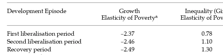
TABLE 6 Summary of Growth and Gini Elasticities of Poverty, 1984–2002
Development Episode Growth
Elasticity of Povertya Elasticity of PovertyInequality (Gini)
First liberalisation period –2.37 0.78 Second liberalisation period –2.46 1.10
Recovery period –2.49 1.30
Entire period –2.43 0.92
a See text for an explanation of ‘growth’ as used in this paper.
Source: Author’s calculations.
fi rst liberalisation period was signifi cantly different from that during the second liberalisation and recovery periods.
When the different development episodes are taken into account, it is
inter-esting to fi nd that the only year dummy coeffi cient that was signifi cant at the
1% level was that for 1996. This is in contrast to the full period estimation, in
which the 2002 dummy coeffi cient was also signifi cant at 1%. This indicates that
growth of mean consumption expenditure per capita and changes in inequality have explained almost all the change in poverty, and that macroeconomic
condi-tions played a role only in 1996. (However, all the coeffi cients on the province
dummies, except that for East Kalimantan – not shown here – are still signifi cant
at the 1% level.) As with the estimates for the full period, so in the individual development episodes, other things being equal, the other 24 provinces on aver-age had estimated head-count poverty ratios lower than that in Papua, in this case by percentages ranging from 24% (Riau) to 81% (South Sulawesi).
Quantifying the growth and inequality effects on poverty
Having measured the magnitude of the growth and inequality elasticities of pov-erty across different development episodes, and knowing the amount of growth
and degree of change in the Gini coeffi cients that actually occurred, it is possible to
calculate the average implied change in poverty resulting from growth (changes
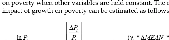
in consumption expenditure) and changes in inequality. For example, the coeffi
-cient
γ
1 in the main poverty equation (equation 1) represents the impact of growthon poverty when other variables are held constant. The magnitude of this partial impact of growth on poverty can be estimated as follows:
lnPt
In the same way, the partial impact of a change in the Gini coeffi cient on
pov-erty can also be estimated:
lnPt
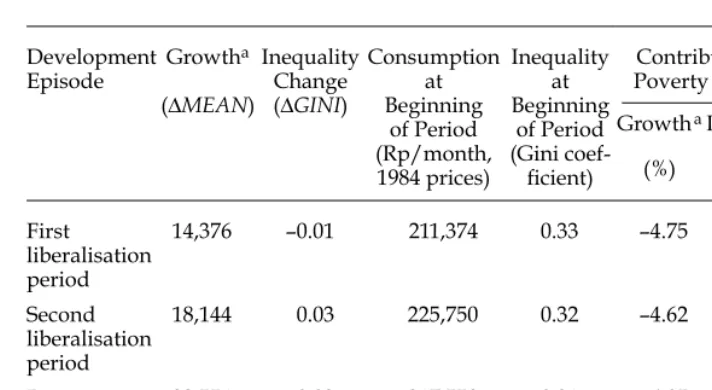
Table 7 shows the respective contributions of growth (as defi ned here) and
change in inequality to the change in national poverty. When we apply the estimated parameters from the regressions above (using the growth and inequality elasticities of poverty shown in table 6), the contribution of growth to the decline in poverty can be seen to be largest during the recovery period, while its lowest contribution was during the second liberalisation period. By contrast, changes in inequality resulted in an offsetting impact on poverty, particularly during the second liberalisation and recovery periods.
The negative impact of change in inequality on poverty during the fi rst liber-alisation period seems credible, given that inequality declined slightly during this period (table 4). The structural transformation away from agriculture and towards labour-intensive manufacturing and services created many new job
opportuni-ties, and this impact was probably more signifi cant for unskilled labour – which is
found near the bottom of the income distribution – thus reducing inequality. The offsetting impact on poverty of changes in inequality during the second
liberalisation period may refl ect the fact that liberalisation had begun to benefi t
the population more widely, rather than mainly just the poor. The Gini coeffi cient
increased rather noticeably during this period (table 4). Further, as a study by Akita and Alisjahbana (2002) reveals, the rapid GDP growth just before the 1997 economic crisis was characterised by increasing within-province inequality, par-ticularly in Riau, and in Jakarta and West and East Java, where the manufactur-ing sector was mainly concentrated. The offsettmanufactur-ing impact of increased inequality on poverty during the recovery period suggests that the recovery might have affected those in transient poverty to a greater extent than those in chronic pov-erty. A thorough examination of the factors that might explain the different signs of the contribution of changes in inequality to poverty changes requires further research, however.
CONCLUSIONS
This paper has used seven waves of the Susenas consumption module to track the dynamics of poverty change across three development episodes. It began with the presumption that different policies followed during each of these episodes could be expected to have differential impacts on poverty during the respective
TABLE 7 Contribution of Growth and Inequality to Change in Poverty
Development
14,376 –0.01 211,374 0.33 –4.75 –0.61 –5.36
Second liberalisation period
18,144 0.03 225,750 0.32 –4.62 2.71 –1.92
Recovery period
22,554 0.02 217,550 0.31 –6.05 2.12 –3.93
Entire period
28,730 0.00 211,374 0.33 –9.74 –0.08 –9.83
a See text for an explanation of ‘growth’ as used in this paper.
Source: Author’s calculations.
periods, especially through the employment effect of labour-intensive growth. Various analysts have argued that, viewed from the demand side, the growth of export-oriented, labour-intensive manufacturing can be seen as one factor among several that help to explain Indonesia’s good record of poverty alleviation since the early 1980s. (At the same time, on the supply side, improvements in education
and health standards have also benefi ted the poor.)
However, our results show that the GEP was remarkably stable across the three development episodes, moving within the narrow range –2.37 to –2.49. The presumption of substantial differences in the GEP between the sub-periods is therefore not supported by the data. By contrast, the inequality elasticity of pov-erty ranged much more widely – between 0.78 and 1.30 – across the development
episodes, with the change between the fi rst and second periods of liberalisation
especially noticeable.
The results also show that change in inequality re-inforced the impact of
growth on poverty only during the fi rst liberalisation period, when inequality
was reduced. In the other two periods, worsening inequality tended to offset the declines in poverty resulting from growth.
Further research will be necessary for a full understanding of these phenom-ena, and will need to control for other explanatory variables that are expected
to infl uence the GEP – in particular, the relevant range of government policies.
The practical reality, however, is that it is diffi cult – perhaps impossible – to fi nd
quantitative measures of the nature of government policies that could be used in analysing the relationship between these policies and changes in inequality, eco-nomic growth and poverty.
REFERENCES
Adams, R.H. Jr (2004) ‘Economic growth, inequality and poverty: estimating the growth elasticity of poverty’, World Development 32 (12): 1,989–2,014.
Akita, T. and Alisjahbana, A.S. (2002) ‘Regional income inequality in Indonesia and the ini-tial impact of the economic crisis’, Bulletin of Indonesian Economic Studies 38 (2): 201–22. Aswicahyono, H. and Feridhanusetyawan, T. (2004) ‘The evolution and upgrading of Indo-nesia’s industry: how can Indonesia maintain its export competitiveness?’, CSIS Work-ing Note 073, Centre for Strategic and International Studies (CSIS), Jakarta.
Balisacan, A.M., Pernia, E.M. and Asra, A. (2003) ‘Revisiting growth and poverty reduction in Indonesia: what do subnational data show’, Bulletin of Indonesian Economic Studies 39 (3): 329–51.
Bidani, B. and Ravallion, M. (1993) ‘A regional poverty profi le for Indonesia’, Bulletin of
Indonesian Economic Studies 29 (3): 37–68.
Bourguignon, F. (2003) ‘The growth elasticity of poverty reduction: explaining heteroge-neity across countries and time periods’, in Growth and Inequality, eds T. Eichler and S. Turnovsky, MIT Press, Cambridge MA.
BPS (Badan Pusat Statistik, Central Statistics Agency) (2003) The Methodology and Poverty Profi le for 2002 [Metodologi dan Profi l Kemiskinan Tahun 2002], BPS, Jakarta.
Datt, G. and Ravallion, M. (1992) ’Growth and redistribution components of changes in poverty measures: a decomposition with applications to Brazil and India in the 1980s’, Journal of Development Economics 38: 275–95.
Deaton, A. (1997) The Analysis of Household Surveys: A Microeconometric Approach to Develop-ment Policy, Johns Hopkins University Press, Baltimore MD.
Deaton, A. (2001) ’Counting the world’s poor: problems and possible solutions’, World Bank Research Observer 16 (2): 125–47.
Deolalikar, A.B. (2002) ‘Poverty, growth and inequality in Thailand’, Asian Development Bank ERD (Economics and Research Department) Working Note Series 8, Asian Devel-opment Bank, Manila.
Fane, G. (1996) ‘Deregulation in Indonesia: two steps forward, one step back’, Agenda 3: 341–80.
Feridhanusetyawan, T. (2002) ‘The social impact of the Indonesian economic crisis: labour market adjustments’, EADN Working Paper, EADN (East Asian Development Net-work) Regional Project on the Social Impact of the Asian Financial Crisis, Institute of Southeast Asian Studies, Singapore.
Friedman, J. (2001) ‘Measuring poverty change in Indonesia, 1984–1996: how responsive is poverty to growth?’, in ‘Essays on Development and Transition’, PhD Thesis, Univer-sity of Michigan, Ann Arbor MI.
Friedman, J. (2005) ‘How responsive is poverty to growth? A regional analysis of poverty, inequality and growth in Indonesia, 1984–1999’, in Spatial Inequality and Development, eds R. Kanbur and A.J. Venables, Oxford University Press, New York NY.
Grimm, M. and Gunther, I. (2006) ‘Growth and poverty in Burkina Fasso: a reassessment of the paradox’, Journal of African Economics16: 70–101.
Hill, H. (1997) Indonesia’s Industrial Transformation, Institute of Southeast Asian Studies, Singapore.
Hill, H. (2000) The Indonesian Economy, 2nd ed., Cambridge University Press, Singapore. Kakwani, N. (1993) ‘Poverty and economic growth with application to Côte d’Ivoire’,
Review of Income and Wealth 39: 121–39.
McLeod, R.H. (1993) ‘Analysis and management of Indonesian money supply growth’, Bulletin of Indonesian Economic Studies 29 (2): 97–128.
Manning, C. (1998) Indonesian Labour in Transition, Cambridge University Press, Cam-bridge.
Manning, C. (2000) ‘Labour market adjustment to Indonesia’s economic crisis: context, trends and implications’, Bulletin of Indonesian Economic Studies 36 (1): 105–36.
Miranti, R. (2007) ‘The Determinants of Regional Poverty in Indonesia: 1984–2002’, PhD dissertation, Australian National University, Canberra.
Miranti, R. and Resosudarmo, B.P. (2005) ’Understanding regional poverty in Indonesia: is poverty worse in the east than in the west?’, Australasian Journal of Regional Studies 11 (2): 141–54.
Nashihin, M. (2007) ‘Poverty Incidence in Indonesia, 1987–2002: A Utility-Consistent Approach Based on a New Survey of Regional Prices’, PhD dissertation, Australian National University, Canberra.
Osmani, S.R. (2004) ‘The employment nexus between growth and poverty: an Asian per-spective’, Report prepared for the Swedish International Development Agency (SIDA), Stockholm, and the United Nations Development Programme (UNDP), New York NY. Ravallion, M. (1994) Poverty Comparisons, Fundamentals in Pure and Applied Economics,
Vol. 56, Harwood Academic Press, Chur, Switzerland.
Ravallion, M. (1995) ‘Growth and poverty: evidence for developing countries in the 1980s’, Economic Letters 48: 411–17.
Ravallion, M. (2001) ‘Growth, inequality and poverty: looking beyond the averages’, World Bank Policy Research Working Paper 2558, World Bank, Washington DC.
Ravallion, M. (2003) ‘Measuring pro-poor growth?’, Economic Letters 78 (1): 93–9.
Ravallion, M. and Chen, S. (1997) ‘What can new survey data tell us about recent changes in distribution and poverty?’, World Bank Economic Review 11 (2): 357–82.
Soesastro, H. (2006) ‘The economic crisis in Indonesia: lessons and challenges for govern-ance and sustainable development’, Pacifi c Link Indonesia, Jakarta, accessed 2 May
2006 at <http://www.pacifi c.net.id/pakar/hadisusastro/economic.html>.
Suryahadi, A. and Sumarto, S. (2001) ’The chronic poor, the transient poor, and the vulner-able in Indonesia before and after the crisis’, SMERU Working Note, SMERU Research Institute, Jakarta.
Suryahadi, A., Sumarto, S. and Pritchett, L. (2003) ‘Evolution of poverty during the crisis in Indonesia’, Asian Economic Journal 17 (3): 221–41
Tarp, F., Simler, K., Matusse, C., Heltberg, R. and Dava, G. (2002) ‘The robustness of pov-erty profi les reconsidered’, Economic Development and Cultural Change 51 (1): 77–108.
Temple, J. (2003) ‘Growing into trouble: Indonesia after 1966’, CEPR Discussion Notes 2932, Centre for Economic Policy Research (CEPR), London.
Wodon, Q.T. (2002) ’Growth, poverty and inequality: a regional panel for Bangladesh‘, World Bank Working Paper 2072, World Bank, Washington DC.
Woo, W.T., Glassburner, B. and Nasution, A. (1994) Macroeconomic Policies, Crises, and Long Term Growth in Indonesia 1965–1990, World Bank, Washington DC.
Wooldridge, J.M. (2003) Introductory Econometrics, 2nd ed., South-Western College Publish-ing, Cincinnati OH.