Full Terms & Conditions of access and use can be found at
http://www.tandfonline.com/action/journalInformation?journalCode=ubes20
Download by: [Universitas Maritim Raja Ali Haji] Date: 11 January 2016, At: 19:51
Journal of Business & Economic Statistics
ISSN: 0735-0015 (Print) 1537-2707 (Online) Journal homepage: http://www.tandfonline.com/loi/ubes20
Forecasting Equity Premium: Global Historical
Average Versus Local Historical Average and
Constraints
Tae-Hwy Lee, Yundong Tu & Aman Ullah
To cite this article: Tae-Hwy Lee, Yundong Tu & Aman Ullah (2015) Forecasting Equity
Premium: Global Historical Average Versus Local Historical Average and Constraints, Journal of Business & Economic Statistics, 33:3, 393-402, DOI: 10.1080/07350015.2014.955174
To link to this article: http://dx.doi.org/10.1080/07350015.2014.955174
Accepted author version posted online: 21 Aug 2014.
Submit your article to this journal
Article views: 130
View related articles
Forecasting Equity Premium: Global Historical
Average Versus Local Historical Average
and Constraints
Tae-Hwy L
EEDepartment of Economics, University of California, Riverside, CA 92521 ([email protected])
Yundong T
UGuanghua School of Management and Center for Statistical Science, Peking University, Beijing, China ([email protected])
Aman U
LLAHDepartment of Economics, University of California, Riverside, CA 92521 ([email protected])
The equity premium, return on equity minus return on risk-free asset, is expected to be positive. We consider imposing such positivity constraint in local historical average (LHA) in nonparametric kernel regression framework. It is also extended to the semiparametric single index model when multiple predictors are used. We construct the constrained LHA estimator via an indicator function which operates as “model-selection” between the unconstrained LHA and the bound of the constraint (zero for the positivity constraint). We smooth the indicator function by bagging, which operates as “model-averaging” and yields a combined forecast of unconstrained LHA forecasts and the bound of the constraint. The local combining weights are determined by the probability that the constraint is binding. Asymptotic properties of the constrained LHA estimators without and with bagging are established, which show how the positive constraint and bagging can help reduce the asymptotic variance and mean squared errors. Monte Carlo simulations are conducted to show the finite sample behavior of the asymptotic properties. In predicting U.S. equity premium, we show that substantial nonlinearity can be captured by LHA and that the local positivity constraint can improve out-of-sample prediction of the equity premium.
KEY WORDS: Bagging; Equity premium; Model averaging; Nonparametric local historical average model; Positivity constraint; Semiparametric single index model.
1. INTRODUCTION
Goyal and Welch (GW,2008) showed that the historical av-erage (HA) forecast of the equity premium (excess return on equity over return on risk-free asset) performs better than fore-casts from the predictive regression using covariates (predic-tors). GW found that numerous economic predictor variables with in-sample significance for the excess stock returns fail to deliver out-of-sample forecasting gains relative to the HA. In GW the benchmark model to beat in out-of-sample forecasting was the “global historical average” (GHA), which is formed from the sample average of the historical equity premium time series over rolling fixed windows or expanding windows.
While the literature has generally confirmed that it is very hard to beat GHA, there are a few limited demonstrations of some success in beating this simple benchmark GHA. In partic-ular we note the following three approaches here. The first one is Campbell and Thompson (CT2008), who asked a question in their article title, “Predicting the equity premium out of sample: Can anything beat the historical average?” They argued that the answer to this question can be “Yes” if theoretically motivated constraints (e.g., monotonicity, positivity) are imposed on the predictive regression function. CT found that the predictive re-gression models with some sensible constraints can do better than GHA. The second one is Hillebrand, Lee, and Medeiros (2014), who used bagging to smooth the CT’s constraint and
found that bagging can further improve CT’s constrained pre-dictive regression forecasts. The third one is Chen and Hong (2009), who showed that the nonparametric nonlinear forecasts are better than the parametric linear regression forecasts.
This article extends the above literature by putting all of these three approaches together. First, following Chen and Hong (2009), we consider nonparametric local models to explore if an LHA model can beat the GHA model.1The answer from our empirical analysis (Section6) is clearly “Yes” using the same dataset used in CT (2008). We find that LHA can easily beat GHA for many predictors (especially for the annualized equity premium in monthly frequency).2Second, following CT (2008), we consider imposing thelocalpositivity constraint on the LHA
1Chen and Hong (2009) used the local linear model, while we use the Nadaraya-Watson local constant model.
2See Section6for the definition of annualized excess return in monthly fre-quency.Qt(k) in Equation (18) withk=12 is the annualized excess return in
montht. Qt(k) withk=1 is the monthly excess return in montht.
© 2015American Statistical Association Journal of Business & Economic Statistics
July 2015, Vol. 33, No. 3 DOI:10.1080/07350015.2014.955174
Color versions of one or more of the figures in the article can be found online atwww.tandfonline.com/r/jbes. 393
equity premium forecast to explore if the constraint can improve the LHA. The answer in Section6is also “Yes” for almost all 11 predictors for the annualized excess returns and also for the monthly excess returns. Third, following Hillebrand, Lee, and Medeiros (2014), we consider bagging to explore if smooth-ing of the constraint can further help the positivity-constrained LHA. The answer given in Section6to this possibility is again “Yes” for most of the 11 predictors for the annualized equity premium and for the monthly excess returns. In summary, these three considerations give us three models—the LHA forecast, the positivity-constrained LHA forecast (denoted as LHAp),
and the bagged positivity-constrained LHA forecast (denoted as LHApb). LHApbis the new equity premium forecast using all
three features (local, constrained, and bagged).
The rest of the article is organized as follows. Section 2
presents four HA models—namely, GHA, LHA, LHAp, and
LHApb. In Section 3 we derive the asymptotic properties of
LHAp (Theorem 1), and LHApb (Theorem 2). We also show
that LHApyields local “model-selection” between LHA model
and the bound of the constraint while LHApb operates as local
“model-averaging” of LHA and the bound of the constraint with the model-averaging weights determined by the probability that the constraint binds (Theorem 3). Extension to models with multivariate predictors is considered in Section 4. Section 5
examines the finite-sample properties of these models via Monte Carlo simulations. Section6evaluates their predictions of equity premium. Section7 concludes. The Appendix collects all the technical proofs.
2. HISTORICAL AVERAGE MODELS
First, we consider the GHA model for the equity premiumy as
is the unconstrained parametric estimator ofα. Note that ˜αis a random variable which is asymptotically normal with meanα.
Now we consider GHA and LHA models for the equity pre-mium. The equity premium is the difference between returns on risky equity and risk-free assets. As the equity premium is the risk premium for the investment on the risky equity, it is expected to be positive, that is α >0. CT (2008) considered imposing such positivity constraint on the linear parametric (global) predictive regression model where the equity premium yis predicted using a predictorx.
We consider such positivity constraint on the LHA model in nonparametric kernel regression framework. Lety be the vari-able to forecast andxbe a predictor. For the ease of exposition, we first consider the LHA model wherexcontains one regressor. The case in which the predictor xis multivariate is treated in Section4. LetIn= {xt−1, yt}nt=1be an observed training sample
(drawn from a stationary process) at timet =nto train the LHA
α(x), andxt is the value ofxat timet.The LHA model is
yt+1=α(xt)+ut+1, (3)
whereα(xt)=E(yt+1|xt),ut+1is a disturbance term such that
E(ut+1|xt)=0 by construction,t =1, . . . , n. The LHA is the local constant kernel estimator ofα(x) trained usingIn
LHA : α(x)˜ = function. ˜α(x) is shown to be asymptotically normal, see Pagan and Ullah (1999). The LHA equity premium forecast at timen using the predictor valuex =xnis ˜α(xn).
We construct the constrained estimator via an indicator func-tion. The indicator function selects either the unconstrained LHA or the bound of the constraint (zero for the positivity constraint) as a forecast of the equity premium. We consider the constraint that the LHA ofyconditional onx,α(x)=E(y|x), exceeds some known lower bound,α1(x). That is,
α(x)> α1(x). (5)
This information is assumed to be known as a prior to a fore-caster. Under this constraint (5), we can easily estimateα(x) with
LHAp : α(x¯ )=α(x)1˜ [ ˜α(x)>α1(x)]+α1(x)1[ ˜α(x)≤α1(x)]. (6)
In the empirical example of this article, we consider the con-straint with the constant bound α1(x)=0, making ¯α(x) the
LHA with positivity constraint (denoted as LHAp). Note that
LHAp operates as local “model-selection” between LHA ˜α(x)
andα1(x)=0 (the martingale difference, MD, model).
The LHAp estimator ¯α(x) involves an indicator and is not
stable in the sense of Breiman (1996b) and B¨uhlmann and Yu (2002). Following B¨uhlmann and Yu (2002), we smooth the indicator function by bagging (Breiman1996a). To define the “bagging positivity-constrained LHA” ofα(x), we construct a bootstrap sample{x∗
t−1, yt∗}nt=1 which is used to derive a
boot-strap constrained estimator via (6) using the plug-in princi-ple. The bagging predictor is an expectation of this estimator over the bootstrapped samples. To be precise, denote ˜α∗(j)(x)
as the unconstrained estimator of α(x) computed from the jth bootstrapped sample {xt∗−(j1), yt∗(j)}nt=1, j=1, . . . , J. Then
the plug-in constrained estimator in the jth bootstrap sample ¯
α∗(j)(x)=α˜∗(j)(x)1[ ˜α∗(j)(x)>α
1(x)]+α1(x)1[ ˜α∗(j)(x)≤α1(x)]. We
de-fine the bagging positivity-constrained LHA estimator (denoted as LHApb) as
in line with that of Breiman (1996a). In the next section, we will show that
ˆ
α(x)≈w(x) ˜α(x)+(1−w(x))α1(x). (8)
In Theorem 3, we show that the combining weight w(x) is the limiting probability that the local positivity-constraint is nonbinding. Ifw(x)>0, bagging operates as convex “model-averaging” locally instead of as “model-selection” and yields a combined forecast of unconstrained LHA ˜α(x) and the bound
Lee, Tu, and Ullah: Forecasting Equity Premium: Global Historical Average Versus Local Historical Average and Constraints 395
of the constraintα1(x). The underlying reason for the benefit
of imposing the (correct) constraint is the “shrinkage” principle with (1−w(x)) being the extent of the shrinkage toward the bound. Breiman (1996a) showed that bagging estimator enjoys a smaller mean squared error loss. B¨uhlmann and Yu (2002) established the asymptotic properties of bagging estimators in variable selection scenario and show that bagging estimator has a much smaller variance, albeit introducing an additional bias. In the next section, we will study sampling properties of LHAp
and LHApb.
3. ASYMPTOTIC PROPERTIES OF LOCAL
HISTORICAL AVERAGE
DenoteZ as a standard normal random variable with CDF (·) and PDFϕ(·). Furthermore, defineZb(x)=Z+b(x). The
following assumptions will be used to establish the asymptotic properties of the constrained estimator and its bagging version.
Assumption A.
Assumption (A.1) places conditions on the bandwidth param-eter. Assumption (A.2) states that the unconstrained estimator
˜
α(x) is asymptotically normal. We note that (A.2) is a high-level assumption whose lower-high-level assumptions would depend on the persistence in the predictor x: (a) when x is strongly mean-reverting (stationary),γ(n, h) is a function of n andh, usually taking the form of√nh. In this case, lower-level as-sumptions that leads to (A.2) can be found in Li and Racine (2007), for example; (b) whenxis highly persistent or unit root, γ(n, h)=
, with convergence in (i) and (iii) of Assumption (A.1) adjusted to convergence in probability, and lower-level assumptions for (A.2) were studied by Bandi (2004), Wang and Phillips (2009a,b) among others. These lower level assumptions are not repeated here. It can be seen that σα(x) represents the asymptotic standard deviation of ˜α(x), whose ex-pression can be found in earlier references. We emphasize that if γ(n, h)h2
→0, the asymptotic bias term of ˜α(x) vanishes to zero. Assumption (A.3) describes that the distance between α(x) and the lower boundα1(x) is controlled by the drift function
b(·). This assumption is only relevant when local asymptotics are considered. It will be made explicit that asymptotic distri-butions of constrained estimators will depend onb(·).
We first establish the following theorem for the constrained estimator ¯α(x).
Theorem 1. (i) Under (A.1)–(A.2), we have,
(a) whenα(x)> α1(x), γ(n, h)σα−1(x)( ¯α(x)−α(x)) d
→Z. (b) when α(x)=α1(x) , Pr[γ(n, h)σα−1(x)( ¯α(x)−α(x))<
z]→d (z)·1{z≥0}.
(ii) If we further assume (A.3), then γ(n, h)σ−1
α (x)( ¯α(x)−α(x)) d
→Zb(x)1[Zb(x)>0]−b(x).
Remark 1. The proofs are collected in the Appendix. Theo-rem 1 states the limiting distribution of ¯α(x). Part (i) presents the usual asymptotic distribution when the constraint is strict and when theα(x) is on the boundary. The result confirms the intuition that, as long as the constraint is strict, it will be met by the unconstrained estimator ˜α(x) when the sample size is large enough. This leads to the conclusion that ¯α(x) would be asymp-totically equivalent to ˜α(x). Whenα(x) is on the boundary, the limiting CDF compresses all the mass of negative values at 0. Part (ii) establishes the local asymptotic distribution of ¯α(x) that depends on the drift parameterb(x). It is easy to see that, ifb(x) is allowed to grow asn,Zb(x)1[Zb(x)>0]−b(x) will collapse toZ,
and result in (ii) becomes that in (i.a). Similarly, (ii)reproduces the result of (i.b) whenb(x)=0.
The following corollary presents the asymptotic bias and vari-ance of the constrained estimator.
Corollary 1. Under (A.1)–(A.3), it follows that
(a) limn→∞γ(n, h)σα−1(x)E[ ¯α(x)−α(x)]=ϕ(b(x))+
Now we consider the LHApbwith the constraint and bagging.
To apply bagging, we need an additional assumption: Assumption A (continued).
(A.4)γ(n, h)σ−1
α (x)( ˜α∗(x)−α(x˜ )) d
→Z.
Assumption (A.4) requires the bootstrap consistency for the unconstrained LHA estimator ˜α(x). Validity for bootstrap for local nonparametric estimators can be found in Hall (1992) or Horowitz (2001).
Theorem 2. Under (A.1)–(A.4), we have,
γ(n, h)σα(x)−1( ˆα(x)−α(x)) d
→Z−Zb(x)(−Zb(x))+
ϕ(−Zb(x)).
Corollary 2. If (A.1)–(A.4) hold, then
(a) limn→∞γ(n, h)σα−1(x)E[ ˆα(x)−α(x)]=2ϕ∗
Remark 2. We adopt the notationf ∗g to denote the con-volution of two functions f and g, defined as f ∗g(s)=
f(t)×g(s−t)dt. Theorem 2 states the limiting distribution of ˆα(x) and Corollary 2 shows the explicit expression for its asymptotic bias and variance. The dependence of the limiting distribution on the drift parameterb(x) is explicit throughZb(x).
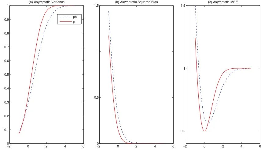
To compare the performance of bagging constrained estimator ˆ
α(x) and constrained estimator ¯α(x) without bagging, we plot asymptotic variance, squared bias and MSE against the drift
functionb(·)=binFigure 1.Figure 1should be understood for GHA or for LHA for a fixed value ofx. We notice from the figure that there is a trade off using bagging, which reduce asymptotic variance while incurring some additional bias. Overall, it is clear that for a large range of values ofb(·) (≥0.391), bagging estimator enjoys a reduction in asymptotic MSE (AMSE).
Theorem 3. Under (A.1)–(A.4), we have
ˆ
α(x)=α(x˜ )(Zb(x))+α1(x)(−Zb(x))+Op
1 γ(n, h) .
Remark 3. Theorem 3 establishes that the LHApb estimator
ˆ
α(x) is a model averaging type estimator with a weight(Zb(x))
assigned to the unconstrained estimator LHA ˜α(x) and a weight (−Zb(x)) to the lower boundα1(x), up to orderOp(γ(n,h1 )). Note that asb(x) increases to infinity, that is, when the constraint be-comes less binding, ˜α(x) will receive probability weight that goes to 1 (since (Zb(x)) approaches 1). On the other hand,
asb(x) decreases to zero, that is, when the constraint becomes more binding,(Zb(x)) will become closer to a uniform random
variable (since(z) is uniform by probability integral transfor-mation). Overall, the performance of the bagging constrained estimator, compared to constrained estimator and unconstrained estimator, can be sensitive to the distance of the lower bound to the true function value, as depicted inFigure 1.
4. SEMIPARAMETRIC EXTENSIONS
In this section, we extend the results developed in the previ-ous section to models with multivariate predictors. It has been long recognized that kernel regressions with multivariate re-gressors suffer from the “curse of dimensionality,” that is, the convergence rate of the kernel estimators will deteriorate as the dimension of the regressors increases. To circumvent this challenge, semiparametric models have become popular. Many recent works have focused on the single index model that en-joys easy implementation. For more details, see Gao (2007) and references therein. This section will illustrate the extension on single index model. We note that the results would be similarly extended to other semiparametric models.
Consider the single index model of the form
yt+1=α(X′tβ0)+ut+1. (9)
The model for iid data has been extensively studied by many authors, to cite a few, Ichimura (1993) and H¨ardle, Hall, and Ichimura (1993). In time series setting, (9) is a special case of the model studied by Xia, Tong, and Li (1999). The esti-mation procedure follows from Ichimura (1993). Let α(z)=
E(yt+1|X′tβ =z). Denote its (leave-one-out) Nadaraya-Watson kernel estimator (with thesth observation omitted) as
˜ tion. The estimation ofβ0and the choice ofhcan be performed
by selecting the orientationβandhthat minimize a measure of the distance. That is, semiparametric single index local historical average forecast at timenusingz=Xn′βˆis obtained from
nβ) to satisfy Assumption (A.1)–(A.2) areˆ given in Xia, Tong, and Li (1999). Under the constraint of (5),
¯ α(X′
nβ) and ˆˆ α(Xn′β) can be defined analogous to (ˆ 6) and (7), respectively. It follows that Theorems 1–3 also hold in the semi-parametric single index model.
5. FINITE SAMPLE PROPERTIES OF LOCAL
HISTORICAL AVERAGE
In this section, we study the finite sample performance of the constrained estimator LHAp α(x) and its bagging version¯ LHApb α(x). We first consider the following data-generatingˆ process (DGP)
Hence, from Assumption (A.3), note that the value ofa also controlsb(x) for givenγ(n, h) andσα(x).We follow the design of Chen and Hong (2009) to allow time series dependence in the predictor and consider different values ofρ chosen from
{0,0.1,0.9,1}. We evaluate the estimators of α(x) at x=1 and 1.5. We compute the mean of squared errors out of 200 Monte Carlo replications. In each replication, we experiment with sample sizen=50,100,200, and the bootstrap sample sizeJ =100 for bagging in each replication. The relative mean squared errors are reported inTable 1. We use cross-validation to select a bandwidth h that minimizes the integrated mean squared error and use this same bandwidth for the J =100 bootstrap samples generated within each replication. The block bootstrap method is used to generate bootstrap samples. We consider the block length to be 1, 4, and 12 but the main results do not change much. Therefore, the result for block length equal to 4 will be reported. See H¨ardle, Horowitz, and Kreiss (2003) and references therein for details of block bootstrap method for time series.
Consider a forecasting model
Model : yt+1=α(x)+ut+1. (15)
For a given evaluation predictor value x, we are inter-ested in forming a forecast ˆyn+1=α(x|In), where In=
Lee, Tu, and Ullah: Forecasting Equity Premium: Global Historical Average Versus Local Historical Average and Constraints 397
−20 0 2 4 6
0.1 0.2 0.3 0.4 0.5 0.6 0.7 0.8 0.9 1
(a) Asymptotic Variance
pb p
−20 0 2 4 6
0.5 1 1.5
(b) Asymptotic Squared Bias
−2 0 2 4 6
0.5 1 1.5
(c) Asymptotic MSE
Figure 1. Asymptotic properties of the local historical average with positivity constraint (LHAp, solid line) and the local historical average with positivity constraint and bagging (LHApb, dashed line).
Monte Carlo average of the squared ˆu(i)(x) overifor each eval-uation pointx,MSE≡ 1
200 200
i=1uˆ
(i)2(x).We compare the three
models pointwise for different values ofx, the results are re-ported inTable 1atx =1 and inTable 2atx =1.5.We report the relative MSE of LHAp α(x) and LHA¯ pb α(x) w.r.t. that ofˆ
LHA ˜α(x).
We summarize the main findings as follows. Atx =1, the constrained estimator works better than unconstrained estima-tor for small values of a in all sample sizes. The gain in relative mean squared errors (MSELHAp/MSELHA) can be as
big as 50%. When a gets larger, the gain of constrained es-timator starts to decrease, as noted by the increase of rela-tive MSE. The constraint will become nonbinding eventually and thus constrained estimator performs the same as the
un-constrained. Bagging does not tend to work for sample size n=50 for small values ofa considered here. When aandn get larger (a =0.02, n=100,200), bagging improves upon the constrained estimator for all values ofρ, with the gain in relative mean squared error (MSELHApb/MSELHA) as large as 5%. This
is consistent with the theory that bagging estimator works better than the constrained estimator when the sample sizenand the level of the function determined byaare of suitable proportion forb(x). For large values ofa, the relative mean squared errors that are larger than 1 are due to sampling errors incurred in the bootstrap procedure.
As shown fromTable 2, the results become more apparent when the estimators are evaluated at x=1.5. Again, the role of the constraint becomes less important asagets larger.
Bag-Table 1. Simulation results for DGP 1: Evaluation point,x=1
n=50 n=100 n=200 n=50 n=100 n=200
a p pb p pb p pb p pb p pb p pb
ρ=0 ρ=0.1
0.001 0.522 0.561 0.556 0.589 0.619 0.644 0.506 0.525 0.624 0.657 0.461 0.483 0.004 0.516 0.539 0.586 0.595 0.572 0.579 0.606 0.633 0.573 0.583 0.534 0.548 0.007 0.644 0.661 0.673 0.657 0.545 0.525 0.670 0.679 0.753 0.766 0.555 0.549 0.010 0.619 0.638 0.707 0.676 0.765 0.725 0.784 0.779 0.720 0.720 0.614 0.598 0.020 0.689 0.681 0.813 0.790 0.818 0.750 0.742 0.715 0.939 0.919 0.745 0.695
ρ=0.9 ρ=1
0.001 0.605 0.634 0.475 0.521 0.538 0.582 0.412 0.356 0.518 0.551 0.587 0.616 0.004 0.550 0.580 0.638 0.663 0.785 0.804 0.481 0.442 0.672 0.712 0.649 0.687 0.007 0.757 0.771 0.610 0.623 0.809 0.813 0.474 0.397 0.811 0.844 0.862 0.901 0.010 0.615 0.623 0.483 0.494 0.946 0.942 0.583 0.447 0.825 0.821 0.895 0.893 0.020 0.707 0.700 0.707 0.697 1.000 0.986 0.743 0.597 0.981 0.897 0.998 0.993
NOTE:aThe column “p” denotes relative MSE of LHA
pto that of LHA and “pb” denotes that of LHApbto LHA.
Table 2. Simulation results for DGP 1: Evaluation point,x=1.5
n=50 n=100 n=200 n=50 n=100 n=200
a p pb p pb p pb p pb p pb p pb
ρ=0 ρ=0.1
0.001 0.555 0.552 0.398 0.389 0.723 0.692 0.534 0.524 0.510 0.489 0.674 0.641 0.004 0.682 0.618 0.759 0.708 0.824 0.715 0.613 0.539 0.607 0.541 0.843 0.763 0.007 0.900 0.802 0.796 0.732 0.957 0.905 0.834 0.754 0.976 0.917 0.990 0.936 0.010 0.997 0.965 0.983 0.920 0.964 0.956 0.8589 0.803 0.982 0.921 1.000 0.999 0.020 1.000 0.995 1.000 0.992 1.000 0.995 1.000 0.972 1.000 0.982 1.000 1.000
ρ=0.9 ρ=1
0.001 0.389 0.404 0.619 0.631 0.717 0.698 0.403 0.392 0.518 0.511 0.452 0.474 0.004 0.681 0.585 0.837 0.796 0.814 0.754 0.407 0.307 0.465 0.342 0.632 0.607 0.007 0.752 0.643 0.948 0.905 0.979 0.912 0.436 0.331 0.563 0.445 0.745 0.650 0.010 0.782 0.702 0.991 0.960 0.968 0.934 0.415 0.295 0.616 0.498 0.877 0.790 0.020 0.987 0.941 1.000 1.010 1.000 0.983 0.660 0.602 0.926 0.759 1.000 0.958
NOTE:aThe column “p” denotes relative MSE of LHA
pto that of LHA and “pb” denotes that of LHApbto LHA.
ging’s role become more salient in this case, with gain in MSE more than 10% whena=0.007 andn=50. AsFigure 1shows, the AMSE of bagging estimator can be over 10% smaller than constrained estimator. So the result we find is congruent with the asymptotic theory. Bagging achieved the maximal amount of gain in relative MSE (16%) when a=0.02, ρ =1 and n=100.
We next consider the following DGP
DGP 2 : yt+1=aexp(xt′β)+et+1, (16)
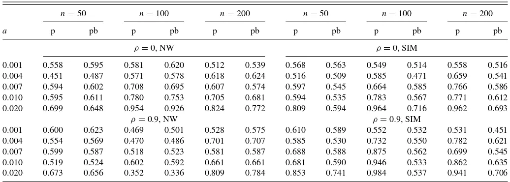
where β =(1,0.5,0.5)′, xt =(x1,t, x2,t, x3,t)′, xk,t, for k= 1,2,3, is generated independently from an AR(1) process as in (14) withµk=1,etanduk,tare iid normal r.v. with mean 0 and σe=1 and σu,k=1, a ∈ {0.001,0.004,0.007,0.010,0.020}. ρ is set to be 0 or 0.9. Other specifications on the simulation are the same as those in DGP 1. We consider two forecasting models. One is the multivariate local constant least square es-timator or the Nadaraya-Watson (NW) eses-timator, and the other is the estimator derived from the single index model (SIM). The models are compared at evaluation point xt=(1,1,1)′.
The relative forecasting MSEs are reported inTable 3. It can be seen from Table 3 that the constrained estimator and the bagging constrained estimator achieve the uniform reduction in MSE for the multivariate NW estimator and the SIM estimator. Furthermore, asagets larger, the bagging constrained estimator tends to outperform the constrained estimator without bagging. The role of imposing constraint becomes less important for largera. These findings are very much similar to those from DGP 1.
6. EMPIRICAL PROPERTIES OF LOCAL
HISTORICAL AVERAGE
To put our proposed constrained local historical average es-timators LHApand LHApbin practice, we consider forecasting
U.S. equity premium. Equity premium or excess return is de-fined as return of the S&P500 Index over the risk-free short-term interest rate. Denote byPt the S&P500 Index at montht. The monthly simple one-month return from monthtto montht+1
Table 3. Simulation results for DGP 2: Evaluation point,x=(1,1,1)′
n=50 n=100 n=200 n=50 n=100 n=200
a p pb p pb p pb p pb p pb p pb
ρ=0, NW ρ=0, SIM
0.001 0.558 0.595 0.581 0.620 0.512 0.539 0.568 0.563 0.549 0.514 0.558 0.516 0.004 0.451 0.487 0.571 0.578 0.618 0.624 0.516 0.509 0.585 0.471 0.659 0.541 0.007 0.594 0.602 0.708 0.695 0.607 0.574 0.597 0.545 0.664 0.585 0.766 0.586 0.010 0.595 0.611 0.780 0.753 0.705 0.681 0.594 0.535 0.783 0.567 0.771 0.612 0.020 0.699 0.648 0.954 0.926 0.824 0.772 0.809 0.594 0.964 0.716 0.962 0.693
ρ=0.9, NW ρ=0.9, SIM
0.001 0.600 0.623 0.469 0.501 0.528 0.575 0.610 0.589 0.552 0.532 0.531 0.451 0.004 0.554 0.569 0.470 0.486 0.701 0.707 0.585 0.530 0.732 0.550 0.782 0.621 0.007 0.599 0.587 0.518 0.523 0.581 0.587 0.688 0.588 0.875 0.562 0.699 0.545 0.010 0.519 0.524 0.602 0.592 0.661 0.661 0.681 0.590 0.946 0.533 0.862 0.635 0.020 0.673 0.656 0.352 0.336 0.809 0.784 0.853 0.741 0.984 0.537 0.941 0.706
NOTE:aThe column “p” denotes relative MSE of LHA
pto that of LHA and “pb” denotes that of LHApbto LHA. NW denotes the Nadaraya-Watson estimator, while SIM denotes the estimator obtained from the single index model.
Lee, Tu, and Ullah: Forecasting Equity Premium: Global Historical Average Versus Local Historical Average and Constraints 399
Table 4. Empirical results
(a) Forecasting annualized equity premiumQt(k=12) at montht
Forecast begins Forecast begins from 1960:01 from 1980:01
LHA LHAp LHApb LHA LHAp LHApb /GHA /GHA /GHA /GHA /GHA /GHA
d/p 0.974 0.963 0.963 0.984 0.975 0.978 e/p 0.979 0.966 0.966 0.990 0.981 0.981 se/p 1.045 1.016 1.009 0.986 0.978 0.976 b/m 1.012 0.999 0.993 1.007 0.997 0.993 roe 1.010 1.000 0.999 1.003 0.999 0.998 t-bill 1.013 0.986 0.983 1.002 0.996 0.993 lty 1.017 0.997 0.989 0.977 0.973 0.971 ts 1.071 1.031 1.017 0.923 0.929 0.932 ds 0.965 0.907 0.899 0.907 0.879 0.871 inf 0.990 0.975 0.979 1.044 1.013 1.008 nei 0.963 0.962 0.962 0.850 0.851 0.848 index 1.006 0.998 0.985 1.033 1.028 1.003
(b) Forecasting monthly equity premiumQt(k=1) at montht
Forecast begins Forecast begins from 1960:01 from 1980:01
LHA LHAp LHApb LHA LHAp LHApb /GHA /GHA /GHA /GHA /GHA /GHA
d/p 1.015 0.993 0.991 0.996 0.994 0.990 e/p 1.028 0.992 0.991 0.993 0.992 0.989 se/p 1.035 1.007 1.003 1.002 1.000 0.996 b/m 1.008 1.004 0.998 0.999 0.999 0.995 roe 1.043 1.021 1.025 1.002 1.000 0.995 t-bill 1.047 1.026 1.015 1.017 1.024 1.002 lty 1.029 1.022 1.008 1.011 1.008 0.998 ts 1.025 1.011 1.024 1.090 1.053 1.046 ds 1.012 1.005 1.009 1.034 1.021 1.022 inf 1.011 0.999 0.997 1.034 1.025 1.023 nei 1.030 1.012 1.007 1.048 1.023 1.008 index 1.023 1.011 1.002 1.024 1.012 1.003
is defined asRt(1)≡Pt+1/Pt−1,and one-month excess return isQt(1)≡Rt(1)−rtwithrt being the risk-free interest rate.
Following Campbell, Lo, and MacKinlay (1997, p. 10), we define thek-period return from monthtto montht+kas
Rt(k)≡
and following CT (2008) we define thek-period excess return as (2008). The results presented inTable 4are with this definition of the equity premium in (18). We have conducted the same analysis withk=3,6 but their results turn out to be what may be easily expected fromk=1,12,and thus we do not report them for space.
We use 11 predictors including dividend price ratio (d/p), earning price ratio (e/p), smooth earning price ratio (se/p), book-to-market ratio (b/m), return on equity (roe), Treasury bill (t-bill), long-term yield (lty), term spread (ts), default spread (ds), inflation (inf) and net equity issuance (nei). We thank John Campbell and Sam Thompson for sharing their data used in CT (2008). It is found thatd/p,e/p,se/p,b/m,roe,t-bill, andltyare unit root processes, while the equity premium (Qt(1), Qt(12)), ts, ds,inf, and nei are not. To save space, we use the first-order difference of the unit root variables when they are used as predictor. The results using the unit root variables (not their differences) as predictors are quite similar and are available from the authors upon request.
We follow CT (2008) to impose a constraint that the eq-uity premium should be positive. We consider the annualized monthly equity premiumQt(12) and monthly equity premium Qt(1),with forecasts starting from 1960:01 and 1980:01 and rolling till 2005:12. The in-sample size for model estimation is kept fixed asR=120. We report the results for mean squared forecast errors (MSFE) relative to the global historical average (GHA) forecast inTable 4.
In Table 4(a) withk=12, we are forecasting the annual-ized equity premiumQt(12) at montht.We first see that non-parametric LHA forecasts ˜α(x) outperform the global histori-cal average GHA ˜α, for the predictord/p,e/p,ds, and neiin both forecasting periods. Second, for these predictors, we ob-serve that imposing the positivity constraint generally reduces the MSFE, which may be further reduced after the bagging procedure. The largest reduction for imposing the constrain oc-curs fords when forecasts begins at 1960:01, and it achieves more than 5%. Third, bagging works for annualized equity pre-mium forecasts for almost all predictors in both forecasting periods, though the improvement is often small. However, this is consistent with the theory in Section 3 as summarized in
Figure 1. Compared to local GHA, the bagging constrained
forecasts are better, except for one case. The maximum gain in MSFE is over 16%, for the predictords, in the forecasting sample 1960:01. Fourth, for the semiparametric single index model that uses all the 11 predictors, the positivity constraint improves the MSFE from 1.006 to 0.998, which is further im-proved by the bagging procedure that achieves a relative MSFE 0.985 when forecasts begins at 1960:01. The similar result in improvement direction is also seen when forecasts begins at 1980:01.
InTable 4(b)withk=1,we are forecasting the monthly eq-uity premiumQt(1) at montht.We hardly see much gain using unconstrained nonparametric methods over the GHA. The best that nonparametric MSFE gains, with 0.7% reduction, is for the predictore/pwhen forecasts start from 1980:01. However, im-posing the positivity constraint LHApalmost always improves MSFE. We observe that bagging works most of the time. Es-pecially for the predictorsd/p,e/p,b/m, bagging even help the nonparametric LHApbforecast to beat the “unbeatable” global
historical average GHA in both forecast samples. This gain is as large as 1.1% fore/pwhen forecasts start from 1980:01, which is economically significant according to Campbell and Thompson (2008).
7. CONCLUSIONS
In this article, we investigate the use of nonparametric lo-cal historilo-cal average and semiparametric single index lolo-cal historical average in forecasting of equity premium, compared to the global historical average which is traditionally used. In addition, we consider imposing a local constraint that the eq-uity premium is expected to be positive. We define the con-strained local historical average forecast and its bagging ver-sion. Asymptotic properties of these constrained/bagged fore-casts are established. We show that the constrained local his-torical average forecast operates as model-selection between the local historical average and zero equity premium, and that the bagged constrained local historical average forecast yields a locally shrunken combined forecast of the local historical average forecast and the zero equity premium forecast. The lo-cal combining weights are determined by the probability that
the local constraint is binding. Significant gains in MSE can be achieved by using a local model, a local constraint, and bagging as shown in our simulation. In predicting U.S. equity premium, we show that substantial nonlinearity is present which can be captured by the nonparametric local historical average and that the local positivity constraint of the equity premium provides valuable prior information in improving its out-of-sample prediction.
The article studies the role of constrained estimation and that of bagging under the condition that the nonparametric estimator is asymptotically normal. In the case of structural change, this condition is often violated. Thus the comparison becomes quite challenging and needs further detailed investigation, which is beyond the scope of this article. Such a potential research topic is left for future study.
Therefore, combining the four terms leads to, (i.a) whenα(x)> α1(x), Pr(γ(n, h)σα−1(x)( ¯α(x)−α(x))< z)→(z) and (i.b) when
Proof of Corollary 1.For a standard normal random variableZand a constantb, we can easily show thatE1[Zb>0]=(b),E[Z1[Zb>0]]=
Lee, Tu, and Ullah: Forecasting Equity Premium: Global Historical Average Versus Local Historical Average and Constraints 401 For the first term in (A.2) we have
γ(n, h)σ−1 Similarly, for the second term in (A.2) we get
γ(n, h)σα−1(x)(α1(x)−α(x))E∗[1[ ˜α∗(x)<α1(x)]]
p
→ −b(x)Z(−Zb(x)), (A.4) by Slutsky’s theorem.
Putting (A.3) and (A.4) together into (A.2) gives the desired result.
Proof of Corollary 2.We can first show thatEϕ(−Zb)=ϕ∗ϕ(−b),
we only need to show that,
E[Z−Zb(x)(−Zb(x))+ϕ(−Zb(x))] Proof of Theorem 3.By definition,
ˆ
Combining the results completes the proof.
ACKNOWLEDGMENTS
The authors thank the Joint Editor (Rong Chen), the Asso-ciate Editor, and three anonymous referees for many valuable suggestions that helped improve the article. Lee and Ullah thank the UCR Academic Senate for research support, and Tu thanks support from Grant 71301004 and Grant 71472007 of National Natural Science Foundation of China.
[Received September 2012. Revised July 2014.]
REFERENCES
Bandi, F. M. (2004), “On Persistence and Nonparametric Estimation,” unpub-lished manuscript, University of Chicago. [395]
Breiman, L. (1996a), “Bagging Predictors,”Machine Learning, 24, 123–140. [394]
——— (1996b), “Heuristics of Instability and Stabilization in Model Selection,” The Annals of Statistics, 24, 2350–2383. [394]
B¨uhlmann, P., and Yu, B. (2002), “Analyzing Bagging,”The Annals of Statistics, 30, 927–961. [394]
Campbell, J. Y., Lo, A. W., and MacKinlay, A. C. (1997),The Econometrics of Financial Markets, Princeton, NJ: Princeton University Press. [399] Campbell, J. Y., and Thompson, S. (2008), “Predicting the Equity Premium
Out of Sample: Can Anything Beat the Historical Average?,”Review of Financial Studies, 21, 1511–1531. [393,394,399]
Chen, Q., and Hong, Y. (2009), “Predictability of Equity Returns Over Differ-ent Time Horizons: A Nonparametric Approach,” working paper, Cornell University. [393,396]
Gao, J. (2007),Nonlinear Time Series: Nonparametric and Semiparametric Methods, London, UK: Chapman & Hall/CRC. [396]
Goyal, A., and Welch, I. (2008), “A Comprehensive Look at the Empirical Performance of Equity Premium Prediction,”Review of Financial Studies, 21, 1455–1508. [393]
Hall, P. (1992),The Bootstrap and Edgeworth Expansion, New York: Springer-Verlag. [395]
H¨ardle, W., Hall, P., and Ichimura, H. (1993), “Optimal Smooth-ing in SSmooth-ingle Index Model,” The Annals of Statistics, 21, 157– 178. [396]
H¨ardle, W., Horowitz, J., and Kreiss, J. P. (2003), “Bootstrap Meth-ods for Time Series,” International Statistical Review, 71, 435– 459. [396]
Hillebrand, E., Lee, T.-H., and Medeiros, M. (2009), “Bagging Constrained Equity Premium Predictors,” inEssays in Nonlinear Time Series Economet-rics, Festschrift in Honor of Timo Ter¨asvirta, eds. N. Haldrup, M. Meitz, and P. Saikkonen, Oxford: Oxford University. [393]
Horowitz, J. L. (2001), “The Bootstrap,” inHandbook of Econometrics(Vol. 5), eds. J. J. Heckman and E. Leamer, Philadelphia: Elsevier. [395] Ichimura, H. (1993), “Semiparametric Least Squares (SLS) and Weighted SLS
Estimation of Single-Index Models,”Journal of Econometrics, 58, 71–120. [396]
Li, Q., and Racine, J. S. (2007),Nonparametric Econometrics, Princeton, NJ: Princeton University Press. [395]
Pagan, A., and Ullah, A. (1999),Nonparametric Econometrics, Cambridge, UK: Cambridge University Press. [394]
Wang, Q., and Phillips, P. C. B. (2009a), “Asymptotic Theory for Local Time Density Estimation and Nonparametric Cointegrating Regression,” Econo-metric Theory, 25, 710–738. [395]
——— (2009b), “Structural Nonparametric Cointegrating Regression,” Econo-metrica, 77, 1901–1948. [395]
Xia, Y., Tong, H., and Li, W. K. (1999), “On Extended Partially Linear Single-Index Models,”Biometrika, 86, 831–842. [396]