EFFICIENT ORIENTATION AND CALIBRATION OF
LARGE AERIAL BLOCKS OF
MULTI-CAMERA PLATFORMS
W. Karel∗, C. Ressl, N. Pfeifer
Department of Geodesy and Geoinformation, TU Wien Gusshausstraße 27-29, 1040 Vienna, Austria
{wilfried.karel, camillo.ressl, norbert.pfeifer}@geo.tuwien.ac.at
KEY WORDS:multi-sensor calibration, oblique aerial imagery, tie point decimation, bundle block adjustment, affine-invariant feature point
ABSTRACT:
Aerial multi-camera platforms typically incorporate a nadir-looking camera accompanied by further cameras that provide oblique views, potentially resulting in utmost coverage, redundancy, and accuracy even on vertical surfaces. However, issues have remained unresolved with the orientation and calibration of the resulting imagery, to two of which we present feasible solutions. First, as standard feature point descriptors used for the automated matching of homologous points are only invariant to the geometric variations of translation, rotation, and scale, they are not invariant to general changes in perspective. While the deviations from local 2D-similarity transforms may be negligible for corresponding surface patches in vertical views of flat land, they become evident at vertical surfaces, and in oblique views in general. Usage of such similarity-invariant descriptors thus limits the amount of tie points that stabilize the orientation and calibration of oblique views and cameras. To alleviate this problem, we present the positive impact on image connectivity of using a quasi affine-invariant descriptor. Second, no matter which hard- and software are used, at some point, the number of unknowns of a bundle block may be too large to be handled. With multi-camera platforms, these limits are reached even sooner. Adjustment of sub-blocks is sub-optimal, as it complicates data management, and hinders self-calibration. Simply discarding unreliable tie points of low manifold is not an option either, because these points are needed at the block borders and in poorly textured areas. As a remedy, we present a straight-forward method how to considerably reduce the number of tie points and hence unknowns before bundle block adjustment, while preserving orientation and calibration quality.
1. INTRODUCTION
While the first aerial photographs in history were oblique, usage of such images has long been limited mostly to visualizations and to object identification in the scope of reconnaissance. However, the combination on a common platform of a nadir-looking cam-era and further camcam-eras that provide oblique views of the ground is potentially beneficiary for geometric reconstruction, because the imagery provides utmost coverage, redundancy, and large in-tersection angles even on otherwise self-occluding surfaces, as found in e.g. highly urbanized and/or vegetated areas.
Given the recent progress in sensor technology, computing hard-ware, and processing automation, usage of aerial multi-camera platforms has become feasible, and they have become commer-cially available, especommer-cially targeting the application of city mod-elling. Most of these systems incorporate a nadir-looking camera and four oblique cameras heading in the four cardinal directions. If their footprints overlap with the one of the nadir camera, then the combined footprint resembles the shape of a Maltese cross, which has given those systems their name.
(Rupnik et al., 2015) show the importance of flight planning for ensuring proper coverage with oblique camera systems of urban canyons, and they demonstrate both with simulations and evalu-ations of real data that the increased redundancy and the larger intersection angles improve the triangulation precision at the ob-ject, especially in the vertical direction.
They use point correspondences only between images of the nadir camera, between oblique images heading in the same direction,
∗Corresponding author
and between images of the nadir and an oblique camera, argu-ing that automatically found putative correspondences between oblique images heading in largely different directions are too prone to be outliers due to respectively large perspective distortions, dif-ferences in image scale, and occlusions. While the decrease in image similarity surely results in a larger ratio of outliers, the question arises whether the categorical rejection of correspon-dences between oblique images of different headings is too con-servative, and thus a considerable amount of them could be used to stabilize the orientation and calibration of the oblique images and cameras. This is particularly important if constant relative orientations of the cameras on the platform are absent e.g. due to a weak mechanical coupling of cameras or a missing synchro-nization of exposures, as repeatedly witnessed by the authors.
Also, (Rupnik et al., 2015) simulate for exemplary cameras the impact of oblique camera tilt and flying overlap on triangulation precision, in order to help with finding a trade-off between costs and data quality. While an increase in overlap beyond 80%/60% per camera does not further improve triangulation precision dra-matically, for city modelling, the overlap may need to be even larger to ensure utmost coverage in complex urban scenes. This means that with oblique multi-camera systems, the number of im-ages to be oriented for a given project area is increased even fur-ther, and this raises the question of how to cope with respectively large bundle block adjustments.
1.1 Feature Matching Facing Large Perspective Distortion SIFT (Lowe, 2004) is probably the most well known feature de-tector and descriptor today. As it searches for local extrema in im-age scale space, it detects stable points that can thus be found re-peatedly under different viewing conditions. By describing their local neighbourhood on that scale and with respect to the lo-cally dominant direction of image gradients, their descriptors are invariant to the geometric transformations of translation, rota-tion, and scale i.e. to a similarity transformation. Thresholding and normalization of the histograms of neighbouring gradients serving as descriptors additionally makes them invariant to lin-ear transformations of image brightness. As all descriptors have the same size and a meaningful Euclidean distance can be de-fined on them, they can be matched efficiently (Muja and Lowe, 2009). While SIFT has proven to work well with a great variety of imagery, the descriptors are not invariant to general changes in perspective and hence, SIFT fails to describe similarly enough corresponding points viewed under largely different perspectives.
In a local neighborhood, even large perspective distortions can be modelled sufficiently by affine transforms, and hence projective-invariant local descriptors would generally be over-parameterized. Thus, research beyond similarity-invariance has concentrated on affine-invariance.
Affine-invariant feature point detectors iteratively adjust their lo-cation, scale, and shape to their local neighbourhood, which may fail, however (Mikolajczyk and Schmid, 2004). Among the affine-invariant region detectors, Maximally Stable Extremal Regions (MSER) (Matas et al., 2002) has proven to be robust. However, its precision is limited, and it depends on extended, planar regions being present on the object.
As an alternative to intrinsically affine-invariant feature point de-tectors, approaches have been proposed that help standard sim-ilarity-invariant feature point detectors to cope with large per-spective distortions. These approaches try to free the imagery be-forehand from distortions that cannot be modelled with similarity transforms, passing respectively warped images on to the detec-tor. If image orientations are approximately known and a coarse object model is available, then the parameters for image warp-ing can be derived directly (see e.g. (Yang et al., 2010)). If that information is missing, then the 2-parameter subspace of affine parameters that similarity-invariant feature detectors are not in-variant to may be sampled, as suggested by (Morel and Yu, 2009) for SIFT, termed Affine-SIFT (ASIFT).
Among other feature detectors, (Apollonio et al., 2014) evaluate SIFT (Lowe, 2004) and ASIFT (Morel and Yu, 2009) for ter-restrial imagery. While they do not find a clear overall winner, we have found ASIFT to work notably well with archaeologial oblique aerial images (Verhoeven et al., 2013).
1.2 Handling Large Bundle Blocks
Once the global rotations are known in a camera network, the camera translations can be derived directly. Thus, methods have been sought after to globally average pairwise camera rotations in a robust way (Hartley et al., 2011, Chatterjee and Govindu, 2013). These methods rely on image features only for the robust compu-tation of relative image oriencompu-tations. Introducing the respective pairwise camera rotations as observations, and using the rotation of one camera as datum, the global rotations of all other cam-eras are adjusted in a first step, without introducing further un-knowns. Subsequently, respective global camera translations are computed, again keeping the translation of one camera fixed, and
without the introduction of any unknowns expect for the transla-tion vectors. While these methods thus broadly increase the max-imum number of images that can be oriented at once and they can provide feasible initial values, global least-squares bundle block adjustment remains the method of choice for the estimation of optimal orientation parameters, self-calibration, and incorpora-tion of addiincorpora-tional observaincorpora-tion types.
Various widely used methods exist that allow for the adjustment of large bundle blocks on finite computing resources. Usage of sparse matrices and the Schur-complement help to lower mem-ory requirements and to speed-up each iteration by splitting the equation system into smaller ones, making use of the structure of the normal equations (Agarwal et al., 2010). Additionally, spe-cialized factorization methods may be used that save memory and work in parallel, e.g. (Chen et al., 2008). Usage of higher-order derivatives reduces the number of needed iterations, and iterative linear solvers further lower the memory requirements, at the cost of introducing a nested loop (Triggs et al., 1999).
However, no matter which hard- and software are used, at some point, a bundle block may comprise too many unknowns to be handled either feasibly or at all. With multi-camera platforms, these limits are reached even sooner. Adjustment of sub-blocks is sub-optimal, as it complicates data management, hinders cam-era calibration, and makes it difficult to estimate globally optimal parameters. No matter which feature point descriptors are in use, the vast majority of tie points will be matched in only 2 views, and these are hence of little reliability. Simply discarding tie points of low manifold randomly is not an option, however, because these points are needed at the block borders and in poorly textured ar-eas. This calls for a method to reduce the number of tie points and hence of unknowns to a large extent, while preserving image orientation and camera calibration quality.
2. METHODS 2.1 Matching Across Oblique Views
We use the quasi-affine-invariant adaptation of SIFT introduced as ASIFT by (Morel and Yu, 2009). Instead of being an intrinsi-cally affine-invariant descriptor, ASIFT feeds the classical SIFT algorithm with affinely warped images. These warped images simulate camera rotations out of the original image plane that hence cannot be modelled with a similarity transform. (Morel and Yu, 2009) suggest to sample this 2-parameter space at 7 po-lar angles from the original optical axis and at an increasing num-ber of equally spaced azimuth angles along a half-circle, starting at 1 (identity) for the zero-polar angle, and ending at 20 for the maximum tilt.
2.2 Decimation of Tie Points
Our goal is to reduce the number of unknowns of a bundle block as much as possible, without compromising image orientation and camera calibration quality notably. Naturally, this calls for a reduction of the number of tie points, especially those that are observed in few images only (low manifold), as they contribute little redundancy.
# Input : # this tie point has been found .
for i m a g e P o i n t in i m a g e P o i n t s :
row , col = g r i d I n d e x ( i m a g e P o i n t . p o s i t i o n ) count = counts [ i m a g e P o i n t . i m a g e I d ] count [ row , col ] += 1
Listing 1: Decimation of tie points in image space in Python-syntax. The definition of the function that computes the grid index associated with an image point position has been omitted.
Extending the approach such that for each camera separately, the tie points with highest manifold in each cell of a grid laid over the project area are kept, leads to a mediocre reduction of the number of tie points, and it may result in unfavourable distributions of image points.
Unlike the aforementioned approaches, the method that we sug-gest to use for the decimation of tie points works in image space instead of object space. Each image is overlaid with a regular grid and a counter for each grid cell. The algorithm then iterates over the tie points sorted by their manifold in descending order. For each tie point, it checks for all of its image points, if the counters for the respective grid cell they fall into is below the minimum number of wanted tie points. If this is not the case for any of its image points, then this tie point will be omitted from bundle ad-justment. Otherwise, the counters of all cells associated with its image points are incremented. The tie point gets scheduled for introduction into the bundle adjustment, and the algorithm pro-ceeds with the next tie point.
Apart from the data, the proposed algorithm requires as input the resolution of the image grid overlay and the minimum number of wanted points per grid cell. Both of these parameters steer the amount of tie point decimation. If no outliers are to be expected in the input data, then the target number of tie points per cell should
be set to 1, which results in most homogeneous distributions of points throughout the image areas.
Listing 1 shows the proposed algorithm in Python code. As can be seen, it is straight-forward, with an outer loop over the sorted list of tie points, and less than two full inner loops over each of their image points. Note that the outer and inner loops may as well be swapped, if that is favourable according to the data structures.
3. EVALUATION
Methods have been implemented in OrientAL (Karel et al., 2013, Karel et al., 2014).
3.1 Similarity- vs. Affine-Invariant Features
For this evaluation, we use scenario “A” of the ISPRS / EuroSDR image orientation benchmark dataset (Nex et al., 2015). From the original imagery, only every other strip has been made available, resulting in 300 images with 60%/60% overlap, all captured in the same flight direction. In addition to the imagery, ground control points at opposite sides of the project area have been published, together with check points with undisclosed object coordinates. Image coordinates of both ground control and check points are provided besides approximate camera interior and exterior orien-tations.
We compare bundle block adjustment results based on the stan-dard SIFT feature point descriptor on the one hand and on its quasi affine-invariant adaptation ASIFT on the other hand. Dur-ing the feature detection stage, the 40k strongest of all detected features are retained per image by both detectors. As we use the parameters suggested by the authors, ASIFT passes for each aerial image 61 warped images on to SIFT, which means that in each warped image, only a fraction of 40k features is retained.
The respective descriptors are then matched with the typical con-straint on mutual nearest neighbors and a threshold on the ra-tio between the descriptor distances to the nearest and second-nearest neighbours. Based on theseinitial matches, relative ori-entations of the image pairs are then computed using RANSAC. Matches that contradict the epipolar constraints are dropped, as are matches that appear to be projected multiply in the same im-age. The chains / connected components of the remaining fil-tered matchesform theinitial tie points. Using these tie points, a robust incremental reconstruction with alternating spatial re-sections and forward interre-sections is executed, during which tie points that contradict the structure are dropped, leaving only the
final tie pointsat the end of reconstruction.
#pairwise matches #image points #object points σ0
init filtered init final init final
SIFT 9510k 237k 2.5% 441k 385k 87% 209k 183k 87% 0.913
ASIFT 6575k 927k 14.1% 1495k 1330k 89% 652k 583k 89% 0.933
Table 1: Efficiency of SIFT vs. ASIFT features.
2 3 4 5 6 7 8 9 10 11 12 13+ Manifold
10-5 10-4 10-3 10-2 10-1 100
Relative Frequency
Tie point manifolds after reconstruction
SIFT
ASIFT
Figure 1: Histograms of tie point manifolds after reconstruction, SIFT vs. ASIFT. The maximum possible manifold would be 25 at the very center of the block (Jacobsen and Gerke, 2016).
reconstruction. However, this is to be expected due to the larger perspective distortions that are coped with.
The higher manifold of ASIFT tie points can also be seen in figure 1. It shows histograms of tie point manifolds at the end of both reconstructions, indicating that indeed ASIFT yields tie points of higher manifolds, albeit the effect is moderate.
Table 2 shows the percentages of tie points at the end of recon-struction that are shared by the 5 cameras, trying to answer the question whether using ASIFT, the goal of increasing the num-ber of tie points in oblique images can be achieved. It turns out that usage of ASIFT increases the ratio of tie points shared by different cameras by a factor of 1.2 to 19.1%, and it increases the fraction of tie points shared by different oblique cameras by a factor of 4, albeit to a still low level of 2%.
3.2 Decimation of Tie Points for Large Bundle Blocks As the dataset used in subsection 3.1 is too small to call for tie point decimation, and as there is hardly any redundant control in-formation publicly available, we use a different data set here that consists of 42k images flown with 70%/60% overlap, taken with 5 Nikon D800E cameras with sensor resolutions of 7360x4912px2 in the classical Maltese cross configuration. They have been cap-tured with unsynchronised camera exposures and along parallel flight strips in mutual flight directions, without cross strips, cov-ering an area of about 27x37km2 of mostly flat terrain. 73 con-trol points are available with according 2717 manual image mea-surements. Feature points detected and matched using Pix4D’s Pix4Dmapper have already been available, and have not been pro-cessed using the method presented in subsection 2.1 due to time constraints.
We decimate the initial 1M tie points using the method presented in subsection 2.2 at decreasing resolutions of grid overlays, each
N E V S W
N 23.61 0.08 1.38 0.03 0.06
E 14.57 9.56 0.17 0.09
V 15.71 2.59 2.06
S sym. 15.10 0.05
W 14.93
(a) SIFT. Different cameras (off-diagonal): 16.1%. Different oblique cameras (off-diagonal, excl. vertical camera): 0.5%.
N E V S W
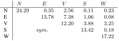
N 24.29 0.35 2.56 0.11 0.23
E 13.78 7.38 1.06 0.08
V 12.20 3.88 3.25
S sym. 13.42 0.18
W 17.22
(b) ASIFT. Different cameras (off-diagonal): 19.1%. Different oblique cameras (off-diagonal, excl. vertical camera): 2.0%.
Table 2: Tie points shared by theVertical and oblique cameras (North,East,South,West) after reconstruction [%], for SIFT (a) and ASIFT (b). Note that tie points with multiplicities larger than 2 contribute to more than 1 entry.
time dropping more and more tie points. As hardly any outliers are to be expected in the data exported from Pix4D, we set the target number of tie points to keep per cell to 1. The grid resolu-tions are selected such that the cells cover approximately square areas, starting at a large resolution with hardly any effect, drop-ping 1 row each time, until reaching the minimum resolution of 3 columns and 2 rows.
Figure 2 shows the effect of tie point decimation on the rela-tive frequency of tie point manifolds: as the algorithm favours tie points of large manifolds, the percentages of large manifolds get increased. Also noticeable is the distribution of manifolds of the tie points delivered by Pix4D, which have obviously been homogenized internally.
The number of remaining tie points decreases smoothly with the decrease of the number of cells in the decimation grid, as can be seen on figure 3. Also, the decimation seems to be efficient, as e.g. a grid with 4 columns and 3 rows that leaves at least 12 points for each image, reduces the number of tie points to 133994, which are only 13% of the original value, and only 3.2 times the number of images.
For evaluating the impact of tie point decimation on the orienta-tion and reconstrucorienta-tion quality, we select 30 control points with 1190 according image points to be used as check points, not to be used in bundle block adjustments. This still leaves 43 con-trol points sparsely distributed across the block that encircle the check points in order to avoid extrapolation, and having accord-ing 1527 image points. For each set of decimated tie points, we run a bundle block adjustment with self-calibration including all parameters of the interior camera orientations and affine, radial, and tangential lens distortion parameters.
5
Tie point manifolds w.r.t. decimation parameters
full5 15x10
5 13x9
5 12x8
5 10x7
5 9x6
5 7x5
5 6x4
5 4x3
0 5 10 15 20 25 30 35 40
5 3x2
Figure 2: Histograms of tie point manifolds [%] at different dec-imation grid resolutions. Top: tie points exported from Pix4D. Bottom: tie points decimated on an image grid overlay with 3 columns and 2 rows. During each decimation process, the target count of tie points per image grid cell to retain is set to 1.
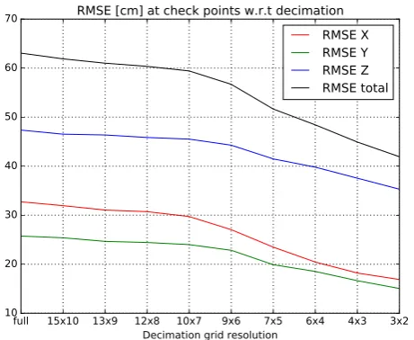
for them. See figure 4 for a plot of the results. As can be expected, RMSEs of Z-coordinates are considerably larger than those of planar coordinates. Noticeable are the consistently larger RMSEs of X-coordinates than those of Y-coordinates. This may be ex-plained by the X-coordinate being parallel to the longer edges of the vertical camera, and hence being parallel to the longer edges of the majority of cameras.
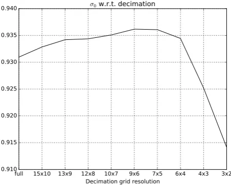
Surprising at first sight is the trend of RMSEs becoming smaller with decreasing numbers of tie points. Comparing this trend with the evolution ofσ0w.r.t. the decimation in figure 5 may provide part of an answer. Whileσ0is increased with a decrease of the number of tie points until a decimation grid resolution of 9x6,σ0 shrinks notably for even smaller grid resolutions and respectively less tie points. This may indicate that by dropping tie points of low manifolds, weakly defined feature points are dropped that do not add significant redundancy, but still affectσ0. However, the relative reduction ofσ0is much smaller than the relative reduc-tion of RMSEs. Apparently, tie points of low manifold have a worse impact on orientation quality than may be derived from the evolution ofσ0. A possible explanation for the large negative in-fluence of low manifold tie points is that their observations are of little reliability and hence, outliers are likely to not be detected.
4. CONCLUSIONS & OUTLOOK
ASIFT features have proven to affect image connectivity posi-tively. They not only increased the average tie point manifold, but they also increased the number of tie points shared between dif-ferent oblique cameras, albeit still on a low level. While ASIFT has been proposed in combination with SIFT, the method of sam-pling camera rotations out of the image plane synthetically be-forehand can be applied to any other similarity-invariant feature point detector. While we have applied it to SIFT only, other de-scriptors are e.g. faster to evaluate, or they provide more compact descriptors, which makes them easier to match.
The demonstrated method for tie point decimation manages to drop large portions of tie points, while increasing the overall tie point manifold, and keeping all images orientable. Furthermore,
full 15x10 13x9 12x8 10x7 9x6 7x5 6x4 4x3 3x2 Decimation grid resolution
0 200000 400000 600000 800000 1000000
1200000
Number of tie points w.r.t decimation
Figure 3: Number of tie points for different decimation grid res-olutions.
full 15x10 13x9 12x8 10x7 9x6 7x5 6x4 4x3 3x2 Decimation grid resolution
10 20 30 40 50 60
70
RMSE [cm] at check points w.r.t decimation
RMSE X
RMSE Y
RMSE Z
RMSE total
Figure 4: RMSE at check points for different decimation grid resolutions.
it is fast, its parameters are easy to understand and memorize, and its implementation may be adapted to the data structures in use. In fact, if the outer loop iterates over the images, then oblique im-ages should be processed first, so to favour their tie points. This would probably homogenize the final count of tie points in the vertical camera and in the oblique cameras. The simplicity and straight-forwardness, however, comes at the cost of not providing globally optimal results, as a considerable number of images will be left with many more tie points than was targeted at.
The possibly surprising correlation of decreasing RMSEs at check points with decreasing numbers of tie points can partly be ex-plained by the likewise decreasingσ0, and the omission of low manifold tie points that are hence of little reliability. However, deficiencies in the data may as well play a role, e.g. missing cross strips and respective difficulties with proper self-calibration.
ACKNOWLEDGEMENTS
full 15x10 13x9 12x8 10x7 9x6 7x5 6x4 4x3 3x2 Decimation grid resolution
0.910 0.915 0.920 0.925 0.930 0.935
0.940 σ0
w.r.t. decimation
Figure 5:σ0for different decimation grid resolutions. Note that
σ0is given in units of a priori standard deviations.
The authors would like to acknowledge the provision of the data-sets by ISPRS and EuroSDR, released in conjuction with the IS-PRS scientific initiative 2014 and 2015, lead by ISIS-PRS ICWG I/Vb.
REFERENCES
Agarwal, S., Snavely, N., Seitz, S. M. and Szeliski, R., 2010. Bundle adjustment in the large. In: Computer Vision–ECCV 2010, Springer, pp. 29–42.
Apollonio, F. I., Ballabeni, A., Gaiani, M. and Remondino, F., 2014. Evaluation of feature-based methods for automated net-work orientation. ISPRS - International Archives of the Pho-togrammetry, Remote Sensing and Spatial Information Sciences XL-5, pp. 47–54.
Chatterjee, A. and Govindu, V., 2013. Efficient and robust large-scale rotation averaging. In: Proceedings of the IEEE Interna-tional Conference on Computer Vision, pp. 521–528.
Chen, Y., Davis, T. A., Hager, W. W. and Rajamanickam, S., 2008. Algorithm 887: Cholmod, supernodal sparse cholesky fac-torization and update/downdate. ACM Trans. Math. Softw. 35(3), pp. 22:1–22:14.
Hartley, R., Aftab, K. and Trumpf, J., 2011. L1 rotation aver-aging using the weiszfeld algorithm. In: Computer Vision and Pattern Recognition (CVPR), 2011 IEEE Conference on, IEEE, pp. 3041–3048.
Jacobsen, K. and Gerke, M., 2016. Sub-camera calibration of a penta-camera. ISPRS - International Archives of the Photogram-metry, Remote Sensing and Spatial Information Sciences XL-3/W4, pp. 35–40.
Karel, W., Doneus, M., Briese, C., Verhoeven, G. and Pfeifer, N., 2014. Investigation on the automatic geo-referencing of ar-chaeological UAV photographs by correlation with pre-existing ortho-photos. ISPRS - International Archives of the Photogram-metry, Remote Sensing and Spatial Information Sciences XL-5, pp. 307–312.
Karel, W., Doneus, M., Verhoeven, G., Briese, C., Ressl, C. and Pfeifer, N., 2013. OrientAL - automatic geo-referencing and ortho-rectification of archaeological aerial photographs. ISPRS Annals of Photogrammetry, Remote Sensing and Spatial Infor-mation Sciences II-5/W1, pp. 175–180.
Lowe, D. G., 2004. Distinctive image features from scale-invariant keypoints. International journal of computer vision 60(2), pp. 91–110.
Matas, J., Chum, O., Urban, M. and Pajdla, T., 2002. Robust wide baseline stereo from maximally stable extremal regions. In: Proceedings of the British Machine Vision Conference, BMVA Press, pp. 36.1–36.10. doi:10.5244/C.16.36.
Mikolajczyk, K. and Schmid, C., 2004. Scale & affine invariant interest point detectors. International Journal of Computer Vision 60(1), pp. 63–86.
Morel, J.-M. and Yu, G., 2009. Asift: A new framework for fully affine invariant image comparison. SIAM Journal on Imaging Sciences 2(2), pp. 438–469.
Muja, M. and Lowe, D. G., 2009. Fast approximate nearest neigh-bors with automatic algorithm configuration. In: International Conference on Computer Vision Theory and Application VISS-APP’09), INSTICC Press, pp. 331–340.
Nex, F., Gerke, M., Remondino, F., Przybilla, H.-J., B¨aumker, M. and Zurhorst, A., 2015. Isprs benchmark for multi-platform photogrammetry. In: ISPRS Annals of the Photogrammetry, Re-mote Sensing and Spatial Information Sciences, Volume II-3/W4. PIA15+HRIGI15 - Joint ISPRS conference 2015, Munich, Ger-many; 2015-03-25 – 2015-03-27.
Rupnik, E., Nex, F., Toschi, I. and Remondino, F., 2015. Aerial multi-camera systems: Accuracy and block triangulation issues. ISPRS Journal of Photogrammetry and Remote Sensing 101, pp. 233 – 246.
Triggs, B., McLauchlan, P. F., Hartley, R. I. and Fitzgibbon, A. W., 1999. Bundle adjustment — a modern synthesis. In: Vi-sion algorithms: theory and practice, Springer, pp. 298–372.
Verhoeven, G., Sevara, C., Karel, W., Ressl, C., Doneus, M. and Briese, C., 2013. Good Practice in Archaeological Diagnostics: Non-invasive Survey of Complex Archaeological Sites. Springer International Publishing, Cham, chapter Undistorting the Past: New Techniques for Orthorectification of Archaeological Aerial Frame Imagery, pp. 31–67.