Full Terms & Conditions of access and use can be found at
http://www.tandfonline.com/action/journalInformation?journalCode=ubes20
Download by: [Universitas Maritim Raja Ali Haji] Date: 12 January 2016, At: 00:16
Journal of Business & Economic Statistics
ISSN: 0735-0015 (Print) 1537-2707 (Online) Journal homepage: http://www.tandfonline.com/loi/ubes20
Testing for Stochastic Dominance Efficiency
Olivier Scaillet & Nikolas Topaloglou
To cite this article: Olivier Scaillet & Nikolas Topaloglou (2010) Testing for Stochastic
Dominance Efficiency, Journal of Business & Economic Statistics, 28:1, 169-180, DOI: 10.1198/ jbes.2009.06167
To link to this article: http://dx.doi.org/10.1198/jbes.2009.06167
Published online: 01 Jan 2012.
Submit your article to this journal
Article views: 163
View related articles
Testing for Stochastic Dominance Efficiency
Olivier S
CAILLETHEC Université de Genève and Swiss Finance Institute, Bd Carl Vogt, 102, CH-1211 Genève 4, Suisse (olivier.scaillet@hec.unige.ch)
Nikolas T
OPALOGLOUDIEES, Athens University of Economics and Business, 76, Patission Str., Athens 104 34, Greece (nikolas@aueb.gr)
We consider consistent tests for stochastic dominance efficiency at any order of a given portfolio with respect to all possible portfolios constructed from a set of assets. We justify block bootstrap approaches to achieve valid inference in a time series setting. The test statistics are computed using linear and mixed integer programming formulations. Monte Carlo results show that the bootstrap procedure performs well in finite samples. The empirical application reveals that the Fama and French market portfolio is first and second-order stochastic dominance efficient, although it is mean–variance inefficient.
KEY WORDS: Block bootstrap; Dominance efficiency; Linear programming; Mixed integer program-ming; Nonparametric; Stochastic ordering.
1. INTRODUCTION
Stochastic dominance is a central theme in a wide vari-ety of applications in economics, finance, and statistics; see, for example, the review papers by Kroll and Levy (1980) and Levy (1992), the classified bibliography by Mosler and Scarsini (1993), and the books by Shaked and Shanthikumar (1994) and Levy (1998). It aims at comparing random variables in the sense of stochastic orderings expressing the common preferences of rational decision makers. Stochastic orderings are binary rela-tions defined on classes of probability distriburela-tions. They trans-late mathematically intuitive ideas like “being larger” or “being more variable” for random quantities. They extend the classical mean–variance approach to compare riskiness.
The main attractiveness of the stochastic dominance ap-proach is that it is nonparametric, in the sense that its criteria do not impose explicit specifications of investor preferences or restrictions on the functional forms of probability distributions. Rather, they rely only on general preference and belief assump-tions. Thus, no specification is made about the return distrib-ution, and the empirical distribution estimates the underlying unknown distribution.
Traditionally, stochastic dominance is tested pairwise. Only recently Kuosmanen (2004) and Post (2003) have introduced the notion of stochastic dominance efficiency. This notion is a direct extension of stochastic dominance to the case where full diversification is allowed. In that setting both authors derive statistics to test for stochastic dominance efficiency of a given portfolio with respect to all possible portfolios constructed from a set of financial assets. Such a derivation relies intrinsically on using ranked observations under an iid assumption on the as-set returns. Contrary to the initial observations, ranked observa-tions, that is, order statistics, are no more iid. Besides, each or-der statistic has a different mean since expectations of oror-der sta-tistics correspond to quantiles. However the approach suggested by Post (2003) based on the bootstrap is valid (see Nelson and Pope1992for an early use of bootstrap in stochastic dominance tests). Indeed, bootstrapping the ranked observations or the ini-tial observations does not affect bootstrap distributions of test statistics, at least in an iid framework.
The goal of this paper is to develop consistent tests for sto-chastic dominance efficiency at anyorder for time-dependent data. Serial correlation is known to pollute financial data (see the empirical section), and to alter, often severely, the size and power of testing procedures when neglected. We rely on weighted Kolmogorov–Smirnov type statistics in testing for stochastic dominance. They are inspired by the consistent pro-cedures developed by Barrett and Donald (2003) and extended by Horvath, Kokoszka, and Zitikis (2006) to accommodate non-compact support. Other stochastic dominance tests are sug-gested in the literature; see, for example, Anderson (1996), Beach and Davidson (1983), and Davidson and Duclos (2000). However these tests rely on pairwise comparisons made at a fixed number of arbitrary chosen points. This is not a desirable feature since it introduces the possibility of test inconsistency. We develop general stochastic dominance efficiency tests that compare a given portfolio with an optimal diversified portfolio formed from a given finite set of assets. We build on the general distribution definition of stochastic dominance in contrast to the traditional expected utility framework.
Note that De Giorgi (2005) solves a portfolio selection prob-lem based on reward-risk measures consistent with second-order stochastic dominance. If investors have homogeneous ex-pectations and optimally hold reward-risk efficient portfolios, then in the absence of market frictions, the portfolio of all in-vested wealth, or the market portfolio, will itself be a reward-risk efficient portfolio. The market portfolio should therefore be itself efficient in the sense of second-order stochastic domi-nance according to that theory (see De Giorgi and Post2008for a rigorous derivation of this result). This reasoning is similar to the one underlying the derivation of the CAPM (Sharpe1964; Lintner1965), where investors optimally hold mean–variance efficient portfolios. A direct test for second-order stochastic dominance efficiency of the market portfolio can be viewed as a nonparametric way to test empirically for such a theory.
© 2010American Statistical Association Journal of Business & Economic Statistics January 2010, Vol. 28, No. 1 DOI:10.1198/jbes.2009.06167
169
The paper is organized as follows. In Section2, we recall the notion of stochastic dominance efficiency introduced by Kuos-manen (2004) and Post (2003), and discuss the general hypothe-ses for testing stochastic dominance efficiency at any order. We describe the test statistics, and analyze the asymptotic proper-ties of the testing procedures. We follow Barrett and Donald (2003) and Horvath, Kokoszka, and Zitikis (2006), who extend and justify the procedure of McFadden (1989) (see also Klecan, McFadden, and McFadden1991; Abadie2002) leading to con-sistent tests of stochastic dominance. We also use simulation based procedures to computep-values. From a technical point of view, we modify their work to accommodate the presence of full diversification and time-dependent data. We rely on a block bootstrap method, and explain this in Section3.
Note that other resampling methods such as subsampling are also available (see Linton, Maasoumi, and Whang2005for the standard stochastic dominance tests). Linton, Post, and Whang (2005) follow this route in the context of testing procedures for stochastic dominance efficiency. They use subsampling to estimate thep-values and discuss power issues of the testing procedures. We prefer block bootstrap to subsampling since the former uses the full sample information. The block boot-strap is better suited to samples with a limited number of time-dependent data; we have 460 monthly observations in our em-pirical application.
Linton, Post, and Whang (2005) focus on the dominance cri-teria of order two and three. In our paper, we also test for first-order stochastic dominance efficiency as formulated in Kuos-manen (2004), although it gives necessary and not sufficient conditions for optimality (Post2005). The first-order stochas-tic dominance criterion places on the form of the utility func-tion no restricfunc-tion beyond the usual requirement that it is non-decreasing, that is, investors prefer more to less. Thus, this criterion is appropriate for both risk averters and risk lovers since the utility function may contain concave as well as con-vex segments. Owing to its generality, the first-order stochas-tic dominance permits a preliminary screening of investment alternatives eliminating those which no rational investor will ever choose. The second-order stochastic dominance criterion adds the assumption of global risk aversion. This criterion is based on a stronger assumption and, therefore, it permits a more sensible selection of investments. The test statistic for second-order stochastic dominance efficiency is formulated in terms of standard linear programming. Numerical implementation of first-order stochastic dominance efficiency tests is much more difficult since we need to develop mixed integer programming formulations. Nevertheless, widely available algorithms can be used to compute both test statistics. We discuss in detail the computational aspects of mathematical programming formula-tions corresponding to the test statistics in Section4.
In Section5we design a Monte Carlo study to evaluate actual size and power of the proposed tests in finite samples. In Sec-tion6we provide an empirical illustration. We analyze whether the Fama and French market portfolio can be considered as effi-cient according to first and second-order stochastic dominance criteria when confronted with diversification principles made of six Fama and French benchmark portfolios formed on size and book-to-market equity ratio (Fama and French1993). The mo-tivation to test for the efficiency of the market portfolio is that
many institutional investors invest in mutual funds. These funds track value-weighted equity indices which strongly resemble the market portfolio. We find that the market portfolio is first and second-order stochastic dominance efficient. We give some concluding remarks in Section7. Proofs and detailed mathe-matical programming formulations are gathered in the Appen-dix.
2. TESTS OF STOCHASTIC DOMINANCE EFFICIENCY
We consider a strictly stationary process {Yt;t∈Z} tak-ing values inRn. The observations consist in a realization of {Yt;t=1, . . . ,T}. These data correspond to observed returns ofnfinancial assets. For inference we also need the process be-ing strong mixbe-ing (α-mixing) with mixing coefficientsαt such that αT =O(T−a)for somea>1 asT → ∞ (see Doukhan
1994 for relevant definition and examples). In particular, re-turns generated by various stationary ARMA, GARCH, and stochastic volatility models meet this requirement (Carrasco and Chen 1998). We denote by F(y) the continuous cdf of
Y=(Y1, . . . ,Yn)′at pointy=(y1, . . . ,yn)′.
Let us consider a portfolioλ∈LwhereL:= {λ∈Rn+:e′λ=
1}withefor a vector made of ones. This means that short sales are not allowed and that the portfolio weights sum to one. Let us denote byG(z,λ;F)the cdf of the portfolio return λ′Yat
From Davidson and Duclos (2000), equation (2), we know that which can be rewritten as
Jj(z,λ;F)= The general hypotheses for testing the stochastic dominance efficiency of orderjofτ, hereafterSDEj, can be written com-pactly as
H0j:Jj(z,τ;F)≤Jj(z,λ;F)
for allz∈Rand for allλ∈L,
H1j:Jj(z,τ;F) >Jj(z,λ;F)
for somez∈Ror for someλ∈L.
In particular, we get first and second-order stochastic domi-nance efficiency whenj=1 and j=2, respectively. The hy-pothesis for testing the stochastic dominance of orderjof the
distribution of portfolioτ over the distribution of portfolioλ
take analoguous forms but for a given λ instead of several of them. The notion of stochastic dominance efficiency is a straightforward extension where full diversification is allowed (Kuosmanen2004; Post2003).
The empirical counterpart to (2.1) is simply obtained by inte-grating with respect to the empirical distributionFˆ ofF, which yields and can be rewritten more compactly forj≥2 as
Jj(z,λ; ˆF)=1 processB◦Fin the space of continuous functions onRn(see, e.g., the multivariate functional central limit theorem for sta-tionary strongly mixing sequences stated in Rio2000), we may derive the limiting behavior of (2.2) using the Continuous Map-ping Theorem (as in lemma 1 of Barrett and Donald2003).
Lemma 2.1. √T[Jj(·; ˆF)− Jj(·;F)] tends weakly to a
For iid data the covariance kernel reduces to
1(z1,z2,λ1,λ2)=E[I{λ′1Y≤z1}I{λ′2Y≤z2}] Let us consider the weighted Kolmogorov–Smirnov type test statistic
and a test based on the decision rule
“rejectHj0ifSˆj>cj,”
wherecj is some critical value that will be discussed in a mo-ment. We introduce the same positive weighting functionq(z)
as in Horvath, Kokoszka, and Zitikis (2006) because we have no compactness assumption on the support ofY. However Hor-vath, Kokoszka, and Zitikis (2006) show that there is no need to introduce it forj=1,2. Then we can takeq(z)=I{z<+∞}. Under that choice ofqthe statement of Proposition2.2below remains true forj=1,2, without the technical assumption on Gneeded for the general result with a higherj.
The following result characterizes the properties of the test, where
¯ Sj:=sup
z,λ
q(z)[Jj(z,τ;B◦F)−Jj(z,λ;B◦F)].
Proposition 2.2. Let cj be a positive finite constant. Let the weighting function q:R→ [0,+∞)satisfy supzq(z)(1+
The result provides a random variable that dominates the lim-iting random variable corresponding to the test statistic under the null hypothesis. The inequality yields a test that never re-jects more often thanα(cj)for any portfolioτsatisfying the null hypothesis. As noted in the result the probability of rejection is asymptotically exactlyα(cj)whenG(z,λ;F)=G(z,τ;F)for allz∈Rand someλ∈L. The first part implies that if we can find acjto set theα(cj)to some desired probability level (say the conventional 0.05 or 0.01) then this will be the significance level for composite null hypotheses in the sense described by Lehmann (1986). The second part of the result indicates that the test is capable of detecting any violation of the full set of restrictions of the null hypothesis.
We conjecture that a similar result holds with supz,λq(z)× Jj(z,λ;B◦F)substituted forS¯j. We have not been able to show this because of the complexity of the covariance of the empiri-cal process which impedes us to exploit the Slepian–Fernique– Marcus–Shepp inequality (see proposition A.2.6 of van der Vaart and Wellner 1996) as in Barrett and Donald (2003). In stochastic dominance efficiency tests this second result would not bring a significant improvement in the numerical tractability as opposed to the context of Barrett and Donald (2003).
In order to make the result operational, we need to find an appropriate critical value cj. Since the distribution of the test statistic depends on the underlying distribution, this is not an
easy task, and we decide hereafter to rely on a block bootstrap method to simulatep-values. The other method suggested by Barrett and Donald (2003), namely a simulation based multi-plier method, would only provide an approximation in our case since it does not work for dependent data.
3. SIMULATIONS OFp-VALUES WITH BLOCK BOOTSTRAP
Block bootstrap methods extend the nonparametric iid boot-strap to a time series context (see Barrett and Donald2003and Abadie2002for use of the nonparametric iid bootstrap in sto-chastic dominance tests). They are based on “blocking” argu-ments, in which data are divided into blocks and those, rather than individual data, are resampled in order to mimick the time-dependent structure of the original data. An alternative resam-pling technique could be subsamresam-pling, for which similar re-sults can be shown to hold as well (see Linton, Maasoumi, and Whang 2005 for use in stochastic dominance tests and com-parison between the two techniques in terms of asymptotic and finite sample properties). We focus on block bootstrap since we face moderate sample sizes in the empirical applications, and wish to exploit the full sample information. Besides, a Monte Carlo investigation of the finite sample properties of subsam-pling based tests is too time consuming in our context (see Sec-tion5on how we solve that problem in a bootstrap setting based on a suggestion of Davidson and MacKinnon2006, 2007).
Letb,ldenote integers such thatT=bl. We distinguish here-after two different ways of proceeding, depending on whether the blocks are overlapping or nonoverlapping. The overlapping rule (Kunsch 1989) produces T −l+1 overlapping blocks, the kth being Bk =(Y′k, . . . ,Y′k+l−1)′ with k∈ {1, . . . ,T − l+1}. The nonoverlapping rule (Carlstein 1986) just asks the data to be divided into b disjoint blocks, the kth being
Bk=(Y′(k−1)l+1, . . . ,Y′kl)′ with k∈ {1, . . . ,b}. In either case the block bootstrap method requires that we choose blocks
B∗1, . . . ,B∗b by resampling randomly, with replacement, from the set of overlapping or nonoverlapping blocks. If B∗i =
(Y∗′i1, . . . ,Y∗′il)′, a block bootstrap sample {Y∗t;t=1, . . . ,T} is made of{Y∗11, . . . ,Y∗1l,Y∗21, . . . ,Y∗2l, . . . ,Y∗b1, . . . ,Y∗bl}, and we letFˆ∗denote its empirical distribution.
Let Eˆ∗ denote the expectation operator with respect to the probability measure induced by block bootstrap sampling. If the blocks are nonoverlapping, then Eˆ∗Jj(z,λ; ˆF∗)=Jj(z,λ; ˆF). In contrast Eˆ∗Jj(z,λ; ˆF∗)=Jj(z,λ; ˆF) under an overlapping scheme (Hall, Horowitz, and Jing1995). The resulting bias de-creases the rate of convergence of the estimation errors of the block bootstrap with overlapping blocks. Fortunately this prob-lem can be solved easily by recentering the test statistic as dis-cussed in Linton, Maasoumi, and Whang (2005) and the review paper of Härdle, Horowitz, and Kreiss (2003) (see also Hall and Horowitz1996and Andrews2002for a discussion of the need for recentering to avoid excessive bias in tests based on extremum estimators). Let us consider
S∗j :=√Tsup z,λ
q(z)[Jj(z,τ; ˆF∗)− ˆE∗Jj(z,τ; ˆF∗)]
− [Jj(z,λ; ˆF∗)− ˆE∗Jj(z,λ; ˆF∗)]
,
with, for the overlapping rule,
ˆ
E∗Jj(z,λ; ˆF∗)= 1
T−l+1 T
t=1
w(t,l,T)
× 1
(j−1)!(z−λ
′Y
t)j−1I{λ′Yt≤z}, where
w(t,l,T)=
t/l ift∈ {1, . . . ,l−1}
1 ift∈ {l, . . . ,T−l+1}
(T−t+1)/l ift∈ {T−l+2, . . . ,T},
and with, for the nonoverlapping rule,Eˆ∗Jj(z,λ; ˆF∗)=Jj(z,
λ; ˆF).
From Hall, Horowitz, and Jing (1995) we have in the over-lapping case
ˆ
E∗Jj(z,λ; ˆF∗)−Jj(z,λ; ˆF)
= [l(T−l−1)]−1[l(l−1)Jj(z,λ; ˆF)−V1−V2], where
V1= l−1
t=1
(l−t) 1
(j−1)!(z−λ
′Y
t)j−1I{λ′Yt≤z} and
V2= T
t=T−l−2
[t−(T−l+1)] 1
(j−1)!(z−λ
′Y
t)j−1I{λ′Yt≤z}, and thus the difference between the two rules vanishes asymp-totically.
Let us define p∗j :=P[S∗j >Sjˆ]. Then the block bootstrap method is justified by the next statement.
Proposition 3.1. Assuming that α < 1/2, a test for SDEj based on the rule
“rejectH0j ifp∗j < α,”
satisfies the following:
limP[rejectH0j] ≤α ifH0j is true,
limP[rejectH0j] =1 ifH0j is false.
In practice we need to use Monte Carlo methods to approx-imate the probability. Thep-value is simply approximated by ˜
pj= R1 Rr=1I{˜Sj,r >Sjˆ}, where the averaging is made on R replications. The replication number can be chosen to make the approximations as accurate as we desire given time and com-puter constraints.
4. IMPLEMENTATION WITH MATHEMATICAL PROGRAMMING
In this section we present the final mathematical program-ming formulations corresponding to the test statistics for first and second-order stochastic dominance efficiency. In the Ap-pendixwe provide the detailed derivation of the formulations.
4.1 Formulation for First-Order Stochastic Dominance
The test statisticSˆ1for first-order stochastic dominance ef-ficiency is derived using mixed integer programming formula-tions. The following is the full formulation of the model:
max z,λ Sˆ1=
√ T1
T T
t=1
(Lt−Wt), (4.1a)
s.t. M(Lt−1)≤z−τ′Yt≤MLt, ∀t, (4.1b) M(Wt−1)≤z−λ′Yt≤MWt, ∀t, (4.1c)
e′λ=1, (4.1d)
λ≥0, (4.1e)
Wt∈ {0,1}, Lt∈ {0,1}, ∀t, (4.1f) withMbeing a large constant.
The model is a mixed integer program maximizing the dis-tance between the sum over all scenarios of two binary vari-ables, T1 Tt=1Lt and T1 Tt=1Wt which represent J1(z,τ; ˆF) andJ1(z,λ; ˆF), respectively (the empirical cdf of portfoliosτ
andλat pointz). According to Inequalities (4.1b),Ltequals 1 for each scenario t∈T for which z≥τ′Yt, and 0 otherwise. Analogously, Inequalities (4.1c) ensure that Wt equals 1 for each scenario for whichz≥λ′Yt. Equation (4.1d) defines the sum of all portfolio weights to be unity, while Inequality (4.1e) disallows for short positions in the available assets.
This formulation permits to test the dominance of a given portfolioτover any potential linear combinationλof the set of other portfolios. So we implement a test of efficiency and not simple stochastic dominance.
When some of the variables are binary, corresponding to mixed integer programming, the problem becomes NP-complete (nonpolynomial, i.e., formally intractible).
The best and most widely used method for solving mixed integer programs is branch and bound (an excellent introduc-tion to mixed integer programming is given by Nemhauser and Wolsey1999). Subproblems are created by restricting the range of the integer variables. For binary variables, there are only two possible restrictions: setting the variable to 0 or setting the vari-able to 1. To apply branch and bound, we must have a means of computing a lower bound on an instance of the optimization problem and a means of dividing the feasible region of a prob-lem to create smaller subprobprob-lems. There must also be a way to compute an upper bound (feasible solution) for at least some in-stances; for practical purposes, it should be possible to compute upper bounds for some set of nontrivial feasible regions.
The method starts by considering the original problem with the complete feasible region, which is called the root problem. The lower-bounding and upper-bounding procedures are ap-plied to the root problem. If the bounds match, then an optimal solution has been found and the procedure terminates. Other-wise, the feasible region is divided into two or more regions, each strict subregions of the original, which together cover the whole feasible region. Ideally, these subproblems partition the feasible region. They become children of the root search node. The algorithm is applied recursively to the subproblems, gen-erating a tree of subproblems. If an optimal solution is found to a subproblem, it is a feasible solution to the full problem,
but not necessarily globally optimal. Since it is feasible, it can be used to prune the rest of the tree. If the lower bound for a node exceeds the best known feasible solution, no globally op-timal solution can exist in the subspace of the feasible region represented by the node. Therefore, the node can be removed from consideration. The search proceeds until all nodes have been solved or pruned, or until some specified threshold is met between the best solution found and the lower bounds on all unsolved subproblems.
In our case, the number of nodes is several hundreds of mil-lions. Under this form, this is a very difficult problem to solve. It takes more than two days to find the optimal solution for rel-atively small time series. We reformulate the problem in order to reduce the solving time and to obtain a tractable formulation. We can see that there is a set of at mostT values, sayR= {r1,r2, . . . ,rT}, containing the optimal value of the variablez. A direct consequence is that we can solve first-order stochastic dominance efficiency by solving the smaller problemsP(r),r∈ R, in whichzis fixed tor. Then we can take the value forzthat yields the best total result. The advantage is that the optimal values of theLtvariables are known inP(r).
The reduced form of the problem is as follows (see the Ap-pendixfor the derivation of this formulation and details on prac-tical implementation):
min T
t=1 Wt,
s.t. λ′Yt≥r−(r−Mt)Wt, ∀t,
e′λ=1, (4.2a)
λ≥0,
Wt∈ {0,1}, ∀t.
4.2 Formulation for Second-Order Stochastic Dominance
The model to derive the test statisticSˆ2for second-order sto-chastic dominance efficiency is the following:
max z,λ Sˆ2=
√ T1
T T
t=1
(Lt−Wt), (4.3a)
s.t. M(Ft−1)≤z−τ′Yt≤MFt, ∀t, (4.3b) −M(1−Ft)≤Lt−(z−τ′Yt)
≤M(1−Ft), ∀t, (4.3c) −MFt≤Lt≤MFt, ∀t, (4.3d) Wt≥z−λ′Yt, ∀t, (4.3e)
e′λ=1, (4.3f)
λ≥0, (4.3g)
Wt≥0,Ft∈ {0,1}, ∀t (4.3h) withMbeing a large constant.
The model is a mixed integer program maximizing the dis-tance between the sum over all scenarios of two variables,
1 T
T
t=1Ltand T1 Tt=1Wtwhich represent theJ2(z,τ; ˆF)and
J2(z,λ; ˆF), respectively. This is difficult to solve since it is the maximization of the difference of two convex functions. We use a binary variable Ft, which, according to Inequalities (4.3b), equals 1 for each scenariot∈Tfor whichz≥τ′Yt, and 0 oth-erwise. Then, Inequalities (4.3c) and (4.3d) ensure that the vari-ableLt equalsz−τ′Yt for the scenarios for which this differ-ence is positive, and 0 for all the other scenarios. Inequalities (4.3e) and (4.3h) ensure thatWt equals exactly the difference z−λ′Ytfor the scenarios for which this difference is positive, and 0 otherwise. Equation (4.3f) defines the sum of all portfolio weights to be unity, while Inequality (4.3g) disallows for short positions in the available assets.
Again, this is a very difficult problem to solve. It takes more than a day for the optimal solution. The model is easily trans-formed to a linear one, which is very easy to solve.
We solve second-order stochastic dominance efficiency by solving again smaller problemsP(r),r∈R, in whichzis fixed tor, before taking the value forzthat yields the best total result.
The new model is the following:
min T
i=1 T
t=1 Wi,t,
s.t. Wi,t≥ri−λ′iYt, ∀i,∀t∈T,
e′λi=1, ∀i, (4.4a)
λi≥0, ∀i, Wi,t≥0, ∀i,∀t.
The optimal portfolioλi and the optimal valueri of variablez are for thati, that gives min Tt=1Wi,t. Now, the computational time for this formulation of the problem is less than a minute.
5. MONTE CARLO STUDY
In this section we design Monte Carlo experiments to evaluate actual size and power of the proposed tests in fi-nite samples. Because of the computational burden of evalu-ating bootstrap procedures in a highly complex optimization environment, we implement the suggestion of Davidson and McKinnon (2006, 2007) to get approximate rejection proba-bilities. We consider two financial assets in a time series con-text. We assume that their returns behave like a stationary vec-tor auvec-toregressive process of order oneYt=A+BYt−1+νt, where νt ∼N(0,) and all the eigenvalues of B are less than one in absolute value. The marginal distribution ofY is Gaussian withμ=(Id−B)−1Aand covariance matrix sat-isfying vec=(Id−B⊗B)−1vec(vecDis the stack of the columns of matrixD).
5.1 Approximate Rejection Probabilities
According to Davidson and MacKinnon (2006, 2007), a sim-ulation estimate of the rejection probability of the bootstrap test at order j and for significance level α is RPˆ j(α) =
1 R
R
r=1I{ˆSj,r <Qˆ∗j(α)} where the test statistics Sˆj,r are ob-tained under the true data generating process onRsubsamples, andQˆ∗j(α)is theα-quantile of the bootstrap statisticsSˆ∗j,r. So, for each one of the two cases (first and second order), the data
generating processDGP0is used to draw realizations of the two asset returns using the vector autoregressive process described above (with different parameters for each case to evaluate size and power). We generateR=300 original samples with size T=460. For each one of these original samples we generate a block bootstrap (nonoverlapping case) data generating process
DGP. OnceDGPis obtained for each replicationr, a new set of random numbers, independent of those used to obtainDGP, is drawn. Then, using these numbers we drawRoriginal samples andRblock bootstrap samples to computeSˆj,r andSˆ∗j,r to get the estimateRPˆ j(α).
5.2 Data Generating Process and Results
To evaluate the actual size, we test for first and second-order stochastic dominance efficiency of one portfolioτ containing the first asset only, that is,τ =(1,0)′, and compare it to all other possible portfoliosλcontaining both assets with positive weights summing to one.
According to Levy (1973, 1982), portfolioτdominates port-folioλ at the first order if μτ > μλ andστ =σλ (with obvi-ous notations). Otherwise we get a crossing. To compute the crossing we solve (x−μτ)/στ =(x−μλ)/σλ. Then we test with a truncation weighting before the crossing, that is, the lowest point across all combinations. By doing so we test on the part of the support where we have strict dominance (see Levy 1982 for the definition of the truncated distributions). We takeA=(0.05,0.05)′, vecB=(0.9,0.1,−0.1,−0.9)′, and vec=(0.1,0,0,0.1)′for the parameters of the vector autore-gressive process. The parameters of the Gaussian stationary dis-tribution are thenμ=(0.5,0)′and vec=(0.5,0,0,0.5)′.
On the other hand, portfolio τ dominates portfolio λ at second order if (μτ −μλ)/(σλ −στ) >0 when μτ > μλ and στ < σλ. We choose here A=(0.05,0.05)′, vecB =
(0.9,0.1,−0.1,−0.9)′, and vec=(0.1,0,0,0.2)′. The pa-rameters of the Gaussian stationary distribution are thenμ=
(0.5,0)′and vec=(0.5,0,0,1)′.
We set the significance levelαequal to 5%, and the block size to l=10. We get RPˆ 1(5%)=4.33% for the first-order stochastic dominance efficiency test, while we getRPˆ 2(5%)= 4.00% for the second-order stochastic dominance efficiency test. Hence we may conclude that both bootstrap tests perform well in terms of size properties.
To evaluate the actual power, we take an inefficient port-folio as the benchmark portport-folioτ, and we compare it to all other possible portfoliosλcontaining both assets with positive weights summing to one. Since portfolioτ is not the efficient one the algorithm should find the first asset of the size design as the efficient one. We use two different inefficient portfolios: the equally weighted portfolio, that is,τ=(0.5,0.5)′, and the portfolio containing the second asset only, that is,τ=(0,1)′.
We find that the power of both tests is large. Indeed, we find ˆ
RP1(5%)=96.66% for the first-order stochastic dominance efficiency test when we take wrongly as efficient the equally weighted portfolio. Similarly, we find RPˆ 1(5%) =97.33% when we take wrongly the second asset as efficient. In the case of the second-order stochastic dominance efficiency, we find
ˆ
RP2(5%)=98.33% andRPˆ 2(5%)=98.66% under the two dif-ferent null hypotheses, respectively.
Table 1. Sensitivity analysis of size and power to the choice of block length. We compute the actual size and power of the first and second-order stochastic dominance efficiency tests for block sizes ranging
froml=4 tol=16. The efficient portfolio isτ=(1,0)′for the size analysis, and eitherτ=(0.5,0.5)′orτ=(0,1)′for
the power analysis
Block sizel 4 8 10 12 16
Size:τ=(1,0)′
ˆ
RP1(5%) 4.00% 4.00% 4.33% 4.00% 5.33%
ˆ
RP2(5%) 3.66% 4.00% 4.00% 4.33% 4.66%
Power:τ=(0.5,0.5)′
ˆ
RP1(5%) 97.66% 97.00% 96.66% 96.66% 95.33% ˆ
RP2(5%) 98.66% 98.33% 98.33% 98.00% 96.33%
Power:τ=(0,1)′
ˆ
RP1(5%) 97.66% 97.00% 97.33% 98.00% 96.66%
ˆ
RP2(5%) 98.33% 98.33% 98.66% 98.66% 97.66%
Finally we present Monte Carlo results in Table1on the sen-sitivity to the choice of block length. We investigate block sizes ranging froml=4 tol=16 by step of 4. This covers the sug-gestions of Hall, Horowitz, and Jing (1995), who show that op-timal block sizes are multiple ofT1/3, T1/4,T1/5, depending on the context. According to our experiments the choice of the block size does not seem to dramatically alter the performance of our methodology.
6. EMPIRICAL APPLICATION
In this section we present the results of an empirical appli-cation. To illustrate the potential of the proposed test statis-tics, we test whether different stochastic dominance efficiency criteria (first and second order) rationalize the market portfo-lio. Thus, we test for the stochastic dominance efficiency of the market portfolio with respect to all possible portfolios con-structed from a set of assets, namely six risky assets. Although we focus the analysis on testing second-order stochastic dom-inance efficiency of the market portfolio, we additionally test for first-order stochastic dominance efficiency to examine the degree of the subject rationality (in the sense that they prefer more to less).
6.1 Description of the Data
We use six Fama and French benchmark portfolios as our set of risky assets. They are constructed at the end of each June,
and correspond to the intersections of two portfolios formed on size (market equity, ME) and three portfolios formed on the ratio of book equity to market equity (BE/ME). The size breakpoint for year t is the median NYSE market equity at the end of June of year t. BE/ME for June of year t is the BE for the last fiscal year end in t−1 divided by the ME for December of t−1. Firms with negative BE are not in-cluded in any portfolio. The annual returns are from January to December. We use data on monthly excess returns (month-end to month-(month-end) from July 1963 to October 2001 (460 monthly observations) obtained from the data library on the homepage of Kenneth French (http:// mba.tuck.dartmouth.edu/ pages/ faculty/ ken.french/ data_library.html). The test portfolio is the Fama and French market portfolio, which is the value-weighted average of all nonfinancial common stocks listed on NYSE, AMEX, and Nasdaq, and covered by CRSP and COM-PUSTAT.
First we analyze the statistical characteristics of the data cov-ering the period from July 1963 to October 2001 (460 monthly observations) that are used in the test statistics. As we can see from Table2, portfolio returns exhibit considerable variance in comparison to their mean. Moreover, the skewness and kurto-sis indicate that normality cannot be accepted for the major-ity of them. These observations suggest adopting the first and second-order stochastic dominance efficiency tests which ac-count for the full return distribution and not only the mean and the variance.
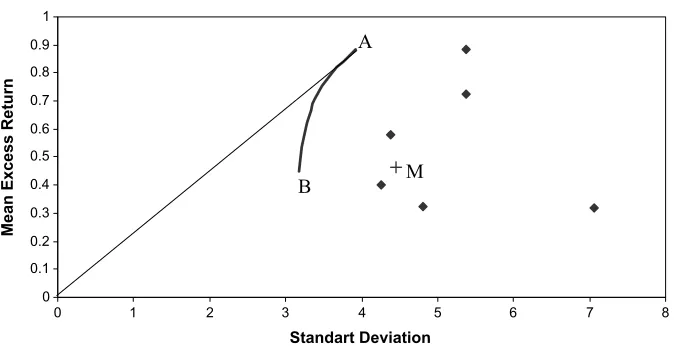
One interesting feature is the comparison of the behavior of the market portfolio with that of the individual portfolios. Fig-ure 1 shows the mean–standard deviation efficient frontier of the six Fama and French benchmark portfolios. The plot also shows the mean and standard deviation of the individual bench-mark portfolio returns and of the Fama and French bench-market (M) portfolio return. We observe that the test portfolio (M) is mean– standard deviation inefficient. It is clear that we can construct portfolios that achieve a higher expected return for the same level of standard deviation, and a lower standard deviation for the same level of expected return. If the investor utility function is not quadratic, then the risk profile of the benchmark portfo-lios cannot be totally captured by the variance of these port-folios. Generally, the variance is not a satisfactory measure. It is a symmetric measure that penalizes gains and losses in the same way. Moreover, the variance is inappropriate to describe the risk of low probability events. Figure1 is silent on return
Table 2. Descriptive statistics of monthly returns in % from July 1963 to October 2001 (460 monthly observations) for the Fama and French market portfolio and the six Fama and French benchmark portfolios formed on size and book-to-market equity ratio. Portfolio 1 has low
BE/ME and small size, portfolio 2 has medium BE/ME and small size, portfolio 3 has high BE/ME and small size, . . . ,
portfolio 6 has high BE/ME and large size
No. Mean Std. dev. Skewness Kurtosis Minimum Maximum
Market portfolio 0.462 4.461 −0.498 2.176 −23.09 16.05
1 0.316 7.07 −0.337 −1.033 −32.63 28.01
2 0.726 5.378 −0.512 0.570 −28.13 26.26
3 0.885 5.385 −0.298 1.628 −28.25 29.56
4 0.323 4.812 −0.291 −1.135 −23.67 20.48
5 0.399 4.269 −0.247 −0.706 −21.00 16.53
6 0.581 4.382 −0.069 −0.929 −19.46 20.46
Figure 1. Mean–standard deviation efficient frontier of six Fama and French benchmark portfolios. The plot also shows the mean and standard deviation of the individual benchmark portfolio returns and of the Fama and French market (M) portfolio return, which is the test portfolio.
moments other than mean–variance (such as higher-order cen-tral moments and lower partial moments). Finally, the mean– variance approach is not consistent with second-order stochas-tic dominance. This is well illustrated by the mean–variance paradox, and motivates us to test whether the market portfolio is first and second-order stochastic dominance efficient. These cri-teria avoid parameterization of investor preferences and the re-turn distribution, and at the same time ensures that the regularity conditions of nonsatiation (first-order stochastic dominance ef-ficiency) and risk aversion (second-order stochastic dominance efficiency) are satisfied. In brief, the market portfolio must be first-order stochastic dominance efficient for all asset pricing models that use a nonsatiable representative investor. It must be second-order stochastic dominance efficient for all asset pricing models that use a nonsatiable and additionally risk-averse rep-resentative investor. This must hold regardless of the specific functional form of the utility function and the return distribu-tion.
6.2 Results of the Stochastic Dominance Efficiency Tests
We find a significant autocorrelation of order one at a 5% significance level in benchmark portfolios 1 to 3, while ARCH effects are present in benchmark portfolio 4 at a 5% significance level. This indicates that a block bootstrap approach should be favored over a standard iid bootstrap approach. Since the au-tocorrelations die out quickly, we may take a block of small size to compute thep-values of the test statistics. We choose a size of 10 observations. We use the nonoverlapping rule be-cause we need to recenter the test statistics in the overlapping rule. The recentering makes the test statistics very difficult to compute, since the optimization involves a large number of bi-nary variables. Thep-values are approximated with an averag-ing made onR=300 replications. This number guarantees that the approximations are accurate enough, given time and com-puter constraints.
For the first-order stochastic dominance efficiency, we can-not reject that the market portfolio is efficient. Thep-valuep˜1=
0.55 is way above the significance level of 5%. We also find that the market portfolio is highly and significantly second-order stochastic dominance efficient sincep˜2=0.59. Although Fig-ure1shows that the market portfolio is inefficient compared to the benchmark portfolios in the mean–variance scheme, the first and second-order stochastic dominance efficiency of the mar-ket portfolio prove the opposite under more general schemes. These results indicate that the whole distribution rather than the mean and the variance plays an important role in comparing portfolios. This efficiency of the market portfolio is interesting for investors. If the market portfolio is not efficient, individual investors could diversify across diverse asset portfolios and out-perform the market.
Our efficiency finding cannot be attributed to a potential lack of power of the testing procedures. Indeed, we use a long enough time series of 460 return observations, and a relatively narrow cross-section of six benchmark portfolios. Further even if our test concerns a necessary and not a sufficient condition for optimality of the market portfolio (Post2005), this does not influence the output of our results. Indeed, the conclusion of the test is that the market portfolio dominates all possible combina-tions of the other portfolios, and this for all nonsatiable decision makers; thus, it is also true for some of them.
6.3 Rolling Window Analysis
We carry out an additional test to validate the second-order stochastic dominance efficiency of the market portfolio and the stability of the model results. It is possible that the efficiency of the market portfolio changes over time, as the risk and prefer-ences of investors change. Therefore, the market portfolio may be efficient in the total sample, but inefficient in some subsam-ples. Moreover, the degree of efficiency may change over time, as pointed by Post (2003). To control that, we perform a rolling window analysis using a window width of 10 years. The test statistic is calculated separately for 340 overlapping 10-year periods, (July 1963–June 1973), (August 1963–July 1973), . . . ,
(November 1991–October 2001).
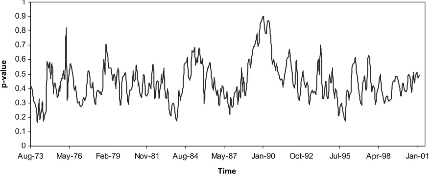
Figure 2. p-values for the second-order stochastic dominance efficiency test using a rolling window of 120 months. The test statistic is calculated separately for 340 overlapping 10-year periods, (July 1963–June 1973), (August 1963–July 1973), . . . , (November 1991–October 2001). The second-order stochastic dominance efficiency is not rejected once.
Figure 2 shows the corresponding p-values. Interestingly, we observe that the market portfolio is second-order stochas-tic dominance efficient in the total sample period. The second-order stochastic dominance efficiency is not rejected on any subsamples. Thep-values are always greater than 15%, and in some cases they reach the 80%–90%. This result confirms the second-order stochastic dominance efficiency that was found in the previous subsection, for the whole period. This means that we cannot form an optimal portfolio from the set of the six benchmark portfolios that dominates the market portfolio by second-order stochastic dominance. The line exhibits large fluctuations; thus the degree of efficiency is changing over time but remains always above the critical level of 5%.
Note that the computational complexity and the associated large solution time of the first-order stochastic dominance effi-ciency test are prohibitive for a rolling window analysis. It in-volves a large number of optimization models: 340 rolling win-dows times 300 bootstraps for each one, times 460 programs, where 460 is the number of discrete values ofz, a discretization that reduces the solution time, as explained in theAppendix.
7. CONCLUDING REMARKS
In this paper we developconsistenttests for stochastic domi-nance efficiency atanyorder fortime-dependentdata. We study tests for stochastic dominance efficiency of a given portfolio with respect to all possible portfolios constructed from a set of risky assets. We justify block bootstrap approaches to achieve valid inference in a time series setting. Linear as well as mixed integer programs are formulated to compute the test statistics.
To illustrate the potential of the proposed test statistics, we test whether different stochastic dominance efficiency criteria (first and second order) rationalize the Fama and French mar-ket portfolio over six Fama and French benchmark portfolios constructed as the intersections of two ME portfolios and three BE/ME portfolios. Empirical results indicate that we cannot re-ject that the market portfolio is first and second-order
stochas-tic dominance efficient. The result for the second order is also confirmed in a rolling window analysis. In contrast, the market portfolio is mean–variance inefficient, indicating the weakness of the variance to capture the risk.
The next step in this line of work is to develop estimators of efficiency lines as suggested by Davidson and Duclos (2000) for poverty lines in stochastic dominance. For the first order we should estimate the smallest return at which the distribu-tion associated with the portfolio under test and the smallest distribution generated by any portfolios built from the same set of assets intersect. Similarly we could rely on an intersection between integrals of these distributions to determine efficiency line at higher orders.
Another future step in this direction is to extend inference procedures to prospect stochastic dominance efficiency and Markowitz stochastic dominance efficiency. These concepts al-low to take into account that investors react differently to gains and losses and haveS-shaped or reverseS-shaped utility func-tions. The development of conditions to be tested for other sto-chastic dominance efficiency concepts is of great interest.
APPENDIX: PROOFS AND MATHEMATICAL PROGRAMMING FORMULATIONS
In the proofs we use the shorter notation Dj(z,τ,λ;F):= Jj(z,τ;F)−Jj(z,λ;F). We often remove arguments, and use to indicate dependence on the empirical distribution. All limits are taken asTgoes to infinity.
A.1 Proof of Proposition2.2
1. Proof of part (i):
By the definition of Sˆj and Dj ≤0 for all z and for all
λ under H0j, we getSjˆ ≤√Tsupq[ ˆDj−Dj] +√TsupqDj ≤ √
Tsupq[ ˆDj−Dj].Writing the latter expression with the sum
of the following six quantities:
A similar equality holds true for the limitSj¯ but based onB◦F instead of√T(Fˆ−F), namely for| ¯θ| ≤1 Then as in Horvath, Kokoszka, and Zitikis (2006) we deduce the weak convergence ofSˆjtoS¯jby lettingLgo to infinity since
only the first supremum in the right-hand side of (A.1) and (A.2) contributes asymptotically under the stated assumptions on q andG.
2. Proof of part (ii):
If the alternative is true, then there exists somezand someλ, say¯z∈Randλ¯∈L, for whichDj(z¯,τ,λ¯;F)=:δ >0. Then the result follows using the inequalitySjˆ ≥q(¯z)√TDj(¯z,τ,λ¯; ˆF), and the weak convergence ofq(·)√T[Dj(·; ˆF)−Dj(·;F)].
A.2 Proof of Proposition3.1
Conditionally on the sample, we have that √
T(Fˆ∗− ˆF)⇒p B∗◦F, (A.3) whereB∗◦Fis an independent copy ofB◦F(Bühlmann1994; Peligrad1998).
We can see that the functionalDj(·;F)is Hadamard differen-tiable atFby induction. IndeedD1(·;F)is a linear functional, whileDj(·;F)is also a linear functional of a Hadamard differ-entiable mappingDj−1(·;F). The delta method (van der Vaart and Wellner1996, chapter 3.9), the continuous mapping theo-rem, and (A.3) then yields
S∗j ⇒p sup z,λ
q(z)Dj(z,τ,λ;B∗◦F), (A.4) where the latter random variable is an independent copy ofS¯j.
Note that the median of the distributionP0j(t)of supz,λq(z)× Dj(z,τ,λ;B′◦F)is strictly positive and finite. Sinceq(z)× Dj(z,τ,λ;B′◦F)is a Gaussian process,P0j is absolutely contin-uous (Tsirel’son1975), whilecj(α)defined byP[¯Sj>cj(α)] = αis finite and positive for anyα <1/2 (proposition A.2.7 of van der Vaart and Wellner1996). The event{p∗j < α}is equiva-lent to the event{ˆSj>c∗j(α)}where
inf{t:P∗j(t) >1−α} =c∗j(α)−→p cj(α), (A.5)
by (A.4) and the aforementioned properties ofP0j. Then
limP[rejectH0j|Hj0] =limP[ˆSj>c∗j(α)]
=limP[ˆSj>cj(α)]
+lim
P[ˆSj>c∗j(α)] −P[ˆSj>cj(α)] ≤P[¯Sj>cj(α)] :=α,
where the last statement comes from (A.5), part (i) of Proposi-tion2.2andcj(α)being a continuity point of the distribution of ¯
Sj. On the other hand part (ii) of Proposition2.2andcj(α) <∞ ensure that limP[rejectHj0|H1j] =1.
A.3 Mathematical Programming Formulations
A.3.1 Formulation for First-Order Stochastic Dominance. The initial formulation for the test statisticSˆ1for first-order sto-chastic dominance efficiency is Model (4.1).
We reformulate the problem in order to reduce the solving time and to obtain a tractable formulation. The steps are the following:
1. The factor√T/T can be left out in the objective function, sinceTis fixed.
2. We can see that there is a set of at most T values, say R= {r1,r2, . . . ,rT}, containing the optimal value of the variablez.
Proof. Vectorsτ andYt,t=1, . . . ,T being given, we can rank the values ofτ′Yt,t=1, . . . ,T, by increasing order. Let us call r1, . . . ,rT the possible different values of τ′Yt, with r1<r2<· · ·<rT (actually there may be less thanT different values). Now, for anyzsuch thatri≤z≤ri+1, t=1,...,TLt is constant (it is equal to the number of t such that τ′Yt ≤ ri). Further, when ri ≤z≤ ri +1, the maximum value of − t=1,...,TWt is reached forz=ri. Hence, we can restrictz to belong to the setR.
3. A direct consequence is that we can solve first-order sto-chastic dominance efficiency by solving the smaller prob-lemsP(r),r∈R, in whichzis fixed tor. Then we take take the value for zthat yields the best total result. The advantage is that the optimal values of the Lt variables are known inP(r). Precisely, t=1,...,TLt is equal to the number oftsuch thatτ′Yt≤r. Hence problemP(r)boils down to
min T
t=1 Wt,
s.t. M(Wt−1)≤r−λ′Yt≤MWt, ∀t∈T,
e′λ=1, (A.6a)
λ≥0,
Wt∈ {0,1}, ∀t∈T.
Note that this becomes a minimization problem.
ProblemP(r)amounts to find the largest set of constraints
λ′Yt≥rconsistent withe′λ=1 andλ≥0.
LetMt=minYt,i,i=1, . . . ,n, that is, the smallest entry of vectorYt.
Clearly, for allλ≥0 such thate′λ=1, we have thatλ′Yt≥ Mt. Hence, problemP(r)can be rewritten in an even better re-duced form:
min T
t=1 Wt,
s.t. λ′Yt≥r−(r−Mt)Wt, ∀t∈T,
e′λ=1, (A.7a)
λ≥0,
Wt∈ {0,1}, ∀t∈T.
We further simplifyP(r)by fixing the following variables: • for alltsuch thatr≤Mt, the optimal value ofWtis equal
to 0 since the half space defined by thetth inequality con-tains the simplex.
• for alltsuch thatr≥Mt, the optimal value ofWtis equal to 1 since the half space defined by thetth inequality has an empty intersection with the simplex.
The computational time for this mixed integer program-ming formulation is significantly reduced. For the optimal so-lution (which involves 460 mixed integer optimization pro-grams, one for each discrete value ofz) it takes less than two hours. The problems are optimized with IBM’s CPLEX solver on an Intel Xeon workstation (with a 2∗2.4 GHz Power, 6 GB of RAM). We note the almost exponential increase in so-lution time with the increasing number of observations. We stress here the computational burden that is managed for these tests. The optimization problems are modeled using two dif-ferent optimization languages: GAMS and AMPL. The Gen-eral Algebraic Modeling System (GAMS) is a high-level mod-eling system for mathematical programming and optimiza-tion. It consists of a language compiler and a stable of inte-grated high-performance solvers. GAMS is tailored for com-plex, large-scale modeling applications. A Modeling Language for Mathematical Programming (AMPL) is a comprehensive and powerful algebraic modeling language for linear and non-linear optimization problems, in discrete or continuous vari-ables
We solve the problem using both GAMS and AMPL. These languages call special solvers (CPLEX in our case) that are spe-cialized in linear and mixed integer programs. CPLEX uses the branch and bound technique to solve the MIP program. The Matlab code (where the simulations run) calls the AMPL or GAMS program, which calls the CPLEX solver to solve the optimization. This procedure is repeated a thousand times for the needs of the Monte Carlo experiments and the empirical ap-plication. The procedure codes are available on request from the authors.
The problems could probably be solved more efficiently by developing specialized algorithms that exploit the structure of the mixed integer programming models. However, issues of im-proving computational efficiency beyond what we manage are not of primary concern in this study.
A.3.2 Formulation for Second-Order Stochastic Dominance. The initial formulation for the test statisticSˆ2for second-order stochastic dominance efficiency is Model (4.3).
We reformulate the problem, following the same steps as for first-order stochastic dominance efficiency. Then the model is transformed to a linear program, which is very easy to solve.
We solve second-order stochastic dominance efficiency by solving again smaller problemsP(r),r∈R, in whichzis fixed tor, before taking the value forzthat yields the best total re-sult. The advantage is that the optimal values of theLtvariables are known inP(r). Precisely,Lt=r−τ′Yt, for the scenarios for which this difference is positive, and zero otherwise. Hence problemP(r)boils down to the linear problem
min T
t=1 Wt,
s.t. Wt≥r−λ′Yt, ∀t∈T,
e′λ=1, (A.8a)
λ≥0,
Wt≥0, ∀t∈T.
The computational time for this linear programming formu-lation is very small. To get the optimal solution (which involves 460 linear optimization programs, one for each discrete value of z) using the CPLEX solver, it takes three minutes on average. We can have an even better formulation of this latter model. Instead of solving it for each discrete time of z, we can re-formulate the model in order to solve for all discrete values ri,i=1, . . . ,T simultaneously. The new model is the
follow-The optimal portfolioλi and the optimal valueri of variablez are for thati, that gives min Tt=1Wi,t. Now, the computational time for this formulation of the problem is less than a minute.
ACKNOWLEDGMENTS
The authors would like to thank Serena Ng, an associate ed-itor, and two referees for constructive criticism and comments which have led to a substantial improvement over the previ-ous version, as well as Thierry Post, Martine Labbé, and Eric Ghysels for their helpful suggestions. Research was financially supported by the Swiss National Science Foundation through NCCR FINRISK. They would also like to thank the participants of the XXXVI EWGFM Meeting on Financial Optimization, Brescia Italy, May 5–7, 2005, of the Workshop on Optimization in Finance, Coimbra Portugal, July 4–8, 2005, and of the Inter-national Conference of Computational Methods in Science and Engineering, Loutraki, Greece, October 21–26, 2005, for their helpful comments.
[Received December 2006. Revised April 2008.]
REFERENCES
Abadie, A. (2002), “Bootstrap Tests for Distributional Treatment Effects in In-strumental Variable Models,”Journal of the American Statistical Associa-tion, 97, 284–292. [170,172]
Anderson, G. (1996), “Nonparametric Tests of Stochastic Dominance in In-come Distributions,”Econometrica, 64, 1183–1193. [169]
Andrews, D. (2002), “Higher-Order Improvements of a Computationally At-tractive k-Step Bootstrap for Extremum Estimators,”Econometrica, 64, 891–916. [172]
Barrett, G., and Donald, S. (2003), “Consistent Tests for Stochastic Domi-nance,”Econometrica, 71, 71–104. [169-172]
Beach, C., and Davidson, R. (1983), “Distribution-Free Statistical Inference With Lorenz Curves and Income Shares,”Review of Economic Studies, 50, 723–735. [169]
Bühlmann, P. (1994), “Blockwise Bootstrapped Empirical Process for Station-ary Sequences,”Annals of Statistics, 22, 995–1012. [178]
Carlstein, E. (1986), “The Use of Subseries Methods for Estimating the Vari-ance of a General Statistic From a Stationary Time Series,”Annals of Sta-tistics, 14, 1171–1179. [172]
Carrasco, M., and Chen, X. (1998), “Mixing and Moment Properties of Various GARCH and Stochastic Volatility Models,”Econometric Theory, 18, 17– 39. [170]
Davidson, R., and Duclos, J.-Y. (2000), “Statistical Inference for Stochastic Dominance and for the Measurement of Poverty and Inequality,” Econo-metrica, 68, 1435–1464. [169,170,177]
Davidson, R., and MacKinnon, J. (2006), “The Power of Bootstrap and Asymp-totic Tests,”Journal of Econometrics, 127, 421–441. [172,174]
(2007), “Improving the Reliability of Bootstrap Tests With the Fast Double Bootstrap,”Computational Statistics & Data Analysis, 51, 3259– 3281. [172,174]
De Giorgi, E. (2005), “Reward–Risk Portfolio Selection and Stochastic Domi-nance,”Journal of Banking and Finance, 29, 895–926. [169]
De Giorgi, E., and Post, T. (2008), “Second Order Stochastic Dominance, Reward–Risk Portfolio Selection and the CAPM,”Journal of Financial and Quantitative Analysis, 43, 525–546. [169]
Doukhan, P. (1994),Mixing: Properties and Examples. Lecture Notes in Statis-tics, Vol. 85, Berlin: Springer. [170]
Fama, E., and French, K. (1993), “Common Risk Factors in the Returns on Stocks and Bonds,”Journal of Financial Economics, 33, 3–56. [170] Hall, P., and Horowitz, J. (1996), “Bootstrap Critical Values for Tests Based on
Generalized-Method-of-Moment Estimators,”Econometrica, 64, 891–916. [172]
Hall, P., Horowitz, J., and Jing, B.-Y. (1995), “On Blocking Rules for the Boot-strap With Dependent Data,”Biometrika, 82, 561–574. [172,175] Härdle, W., Horowitz, J., and Kreiss, J.-P. (2003), “Bootstrap Methods for Time
Series,”International Statistical Review, 71, 435–459. [172]
Horvath, L., Kokoszka, P., and Zitikis, R. (2006), “Testing for Stochastic Dom-inance Using the Weighted McFadden-Type Statistic,”Journal of Econo-metrics, 133, 191–205. [169-171,178]
Klecan, L., McFadden, R., and McFadden, D. (1991), “A Robust Test for Sto-chastic Dominance,” working paper, Dept. of Economics, MIT. [170] Kroll, Y., and Levy, H. (1980), “Stochastic Dominance Criteria: A Review and
Some New Evidence,” inResearch in Finance, Vol. II, Greenwich: JAI Press, pp. 263–227. [169]
Kunsch, H. (1989), “The Jackknife and the Bootstrap for General Stationary Observations,”Annals of Statistics, 17, 1217–1241. [172]
Kuosmanen, T. (2004), “Efficient Diversification According to Stochastic Dom-inance Criteria,”Management Science, 50, 1390–1406. [169-171] Lehmann, E. (1986),Testing Statistical Hypotheses(2nd ed.), New York: Wiley.
[171]
Levy, H. (1973), “Stochastic Dominance Among Lognormal Prospects,” Inter-national Economic Review, 14, 601–614. [174]
(1982), “Stochastic Dominance Rules for Truncated Normal Distrib-utions: A Note,”Journal of Finance, 37, 1299–1303. [174]
(1992), “Stochastic Dominance and Expected Utility: Survey and Analysis,”Management Science, 38, 555–593. [169]
(1998),Stochastic Dominance, Boston: Kluwer Academic. [169] Lintner, J. (1965), “Security Prices, Risk and Maximal Gains From
Diversifica-tion,”Journal of Finance, 20, 587–615. [169]
Linton, O., Maasoumi, E., and Whang, Y.-J. (2005), “Consistent Testing for Stochastic Dominance Under General Sampling Schemes,”Review of Eco-nomic Studies, 72, 735–765. [170,172]
Linton, O., Post, T., and Whang, Y.-J. (2005), “Testing for Stochastic Domi-nance Efficiency,” working paper, LSE. [170]
McFadden, D. (1989), “Testing for Stochastic Dominance,” inStudies in the Economics of Uncertainty, eds. T. Fomby and T. Seo, New York: Springer-Verlag, pp. 113–134. [170]
Mosler, K., and Scarsini, M. (1993),Stochastic Orders and Applications, a Classified Bibliography, Berlin: Springer-Verlag. [169]
Nelson, R., and Pope, R. (1992), “Bootstrapped Insights Into Empirical Appli-cations of Stochastic Dominance,”Management Science, 37, 1182–1194. [169]
Nemhauser, G., and Wolsey, L. (1999),Integer and Combinatorial Optimiza-tion, New York: Wiley. [173]
Peligrad, M. (1998), “On the Blockwise Bootstrap for Empirical Processes for Stationary Sequences,”Annals of Probability, 26, 877–901. [178] Post, T. (2003), “Empirical Tests for Stochastic Dominance Efficiency,”Journal
of Finance, 58, 1905–1031. [169-171,176]
(2005), “Wanted: A Test for FSD Optimality of a Given Portfolio,” working paper, Erasmus University. [170,176]
Rio, E. (2000),Théorie Asymptotique des Processus Aléatoires Faiblement Dépendants. Mathématiques et Applications, Vol. 31, Berlin: Springer-Verlag. [171]
Shaked, M., and Shanthikumar, J. (1994),Stochastic Orders and Their Appli-cations, New York: Academic Press. [169]
Sharpe, W. (1964), “Capital Asset Prices: A Theory of Market Equilibrium Un-der Conditions of Risk,”Journal of Finance, 19, 425–442. [169]
Tsirel’son, V. (1975), “The Density of the Distribution of the Maximum of a Gaussian Process,”Theory of Probability and Their Applications, 16, 847– 856. [178]
van der Vaart, A., and Wellner, J. (1996),Weak Convergence and Empirical Processes, New York: Springer-Verlag. [171,178]