Wind Affected Density Current Profile in a Small Semi-Enclosed
Water Body
Purwanto, B. S.1
Abstract: Density current is a type of current that occurs when fluid flow enters a fluid body of different density. The density difference introduces stratification state that requires treatment in the parameterization of turbulence. Due to the geometric shape of location of this study, which is considerably small semi-enclosed water body, a Quasi-Equilibrium Turbulent Energy (QETE) model was selected. QETE was selected because of its convenient parameterization of wind induced breaking wave effect on turbulence. Two equations of the model, turbulence kinetic energy and turbulence macro length scale, were discretized and implemented into a three-dimensional hydrodynamic model. Application to density current simulation in the location of study was then carried out using the resulted model. To show how effective formulation of wind induced breaking wave effect would be, three parameterizations of turbulence were considered. They include QETE model with and without breaking wave effect boundary conditions (BC), and constant eddy viscosity turbulence parameterizations. It was clear from the simulation results that wind induced breaking-wave effect on the density current is quite significant.
Keywords: density current, two-equation turbulence model, wind induced breaking-wave, semi-enclosed water body, numerical simulation.
Introduction
Formation of density current (also called gravity or buoyancy currents) basically happens when fluid flow enters a fluid body of different density. It can happen in many types of nature including limnology, oceanography, and meteorology. Study of density current can be focused on many aspects depending on which environment the current occurs. In a lake nearby a sea or in a coastal lagoon, which has connection with the open sea, salinity may become the key factor introducing the density current. It often has impact on distribution of living organism and water exchange. In Nagatsura-ura lagoon, the location of study, intrusion of sea water occurs and affects mixing mechanism depending on the degree of inflowing salinity. Inflowing salinity into the lagoon varies due to the influence of the Kitakami River discharges and wind conditions [1]. The density currents flowing into the lagoon can be a major source of mixing and exchange processes within the water body.
1 Civil Engineering Department, Universitas Jenderal Soedirman Email: [email protected]
Note: Discussion is expected before June, 1st 2009, and will be published in the “Civil Engineering Dimension” volume 11, number 2, September 2009.
Received 26 September 2008; revised 14 January 2009; accepted 17 February 2009.
Therefore, from both the management and modeling perspective, reproduction of the current through numerical simulation is crucial. One aspect that should be considered in the current reproduction is turbulence closure modeling that calculates effect of stratification on turbulence.
In engineering perspective that is mainly interested only on mean flow quantities, turbulence closure modeling could be an important factor in successful computation of various kinds of flow and transport problems. The closure modeling needs a turbulence model, which is defined as a set of equations (algebraic or differential) that determine the tur-bulent transport terms in the mean-flow equations and thus close the system equations [2]. Turbulence models are classified based on complexity of their formulation. Most of them are based on Boussinesq assumption that relates Reynolds stress tensor to velocity gradient via the turbulent viscosity/ diffusivity. They, in increasing order of complexity, are algebraic models, one-equation models, and two-equation models. Basically, more complex model considers more physical phenomena and therefore more general problem can be handled.
efficient and reasonably accurate. Recently, there are several two-equation models available to be imple-mented into water flow calculation problems. Among
them, the Rodi’s k-ε [3] and Mellor and Yamada [4]
are the two that are often confronted to each other [5, 6]. They are also confronted with other turbulence closure scheme [7-11]. Comparative studies of turbulence model application in estuaries and shallow water environment that have been done so far, however, generally show almost similar perfor-mance among the models considered [12]. Therefore, choice among them is sometimes a matter of practical applicability of the model associated with a problem considered.
In this paper, QETE (Quasi-Equilibrium Turbulent Energy) model [13], which is still in the family of Mellor Yamada turbulence closure [4], is solved numerically and implemented into a three dimen-sional hydrodynamic model. The QETE consists of two partial differential equations for turbulence
kinetic energy q2/2, and a turbulence macro length
scale l. The model has the benefit of easily
incur-porating wind induced breaking wave effect in the formulation. Other two equations turbulence closure
method, i.e. k-ε method, needs more complicated
modification of the original equation to take into account the effect [14]. Considering geometric shape of the location of study combined with continuously blown wind condition during the simulation period, the turbulent model requires formulation of wave-induced breaking wave effect. Therefore, The QETE model is expected to be suitably applied to density current simulation in Nagatsura-ura lagoon, Japan. To show how effective formulation of wind induced breaking wave effect will be, three parameterizations of turbulence are considered. They include QETE model with and without breaking wave effect boundary conditions (BC), and constant eddy visco-sity turbulence parameterizations.
Method
The Turbulence Model
The QETE model calculates eddy viscosity, νv and
eddy diffusivity, Kv by the expressions
m
the macro length scale of turbulence. The stability functions as stated in Blumberg et al. [15] are
(
)(
)
kinetic energy is calculated from
⎥
is shear production;
z
Turbulence length scale l is determined from
differential equation as suggested by Blumberg et al. [15]
surface. Galperin et al. [13] found that it is necessary to limit the length scale using the expression
N q
l≤0.53 (9)
To take into account the effect of breaking wave at the water surface, the vertical boundary condition of turbulence kinetic energy imposed at the water surface is the one suggested by Mellor and Blumberg [16]
which is the alternate version of the Craig and
Banner [17] relation. In the formulation, αCB is Craig
and Banner constant and uτ is water side friction
velocity. Commonly, at the absent of breaking wave effect, assumption for surface boundary condition of turbulent kinetic energy uses relation as proposed by
Mellor and Yamada [4], i.e. q2=Bl2/3(u
τ)2. Moreover,
boundary condition for the length scale at water surface also differs from the common assumption, i.e.
q2l=0, by inclusion of surface roughness length
s
z
l
=
κ
(11)where κ is von-Karman’s constant (≅0.41); and zs is
the surface roughness length. It is noted by Craig
and Banner [17] that feasible values of zs are within
(
)
( )
2where h0 is water depth measured from the
undis-turbed free surface. First order upwind scheme is used to discretize advection terms in Eq. (5) and Eq. (8), whereas the remaining terms are discretized by following the work of Gross et al. [18].
Numerical Discretization
Neglecting the advection terms, Gross et al. [18] discretized the turbulent kinetic energy equation (Eq. 5) and turbulent macro length scale (Eq. 8) of the QETE model to incorporate it into TRIM (Tidal, Residual, and Intertidal Mudflat) 3D model of Casulli and Cheng [19]. The present 3D hydrody-namics model is similar in formulation to TRIM 3D model. Detail discretization of the hydrodynamics model can be found elsewhere [20]. However, to implement the discrete forms of the turbulence model, some modifications are necessary because the present model implements vertical layers numbering that increasingly starts from surface to bottom, which is in opposite direction with the one used in TRIM 3D model. Variables arrangements of the turbulence parameters locate at the same place as vertical flow velocity w. Their locations are schematically shown in Fig. 1.
q2k, qlk
Figure 1. Vertical variables arrangements of the turbu-lence parameters
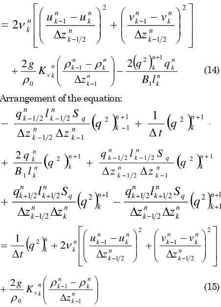
After adjustment to match the present code, the discrete form of Eq. (5) without the advection terms is
Arrangement of the equation:
( )
1( )
2 1Equation (15) is a tridiagonal system of linear equations, which can be solved efficiently using Thomas Agorithm [21].
The other equation, i.e. the turbulent macroscale equation Eq. (8), without the advection terms, is discretized similarly as in Gross et. al. [18] and is adjusted to match the present code. The result is
Arrangement of the equation results in
Similar as for Eq. (7-15), Eq. (17) is then solved using the Thomas Algorithm [21].
As for the advection terms in Eq. (5) and Eq. (8), first order upwind scheme is implemented. Advection terms are discretized implicitly in vertical and explicitly in horizontal. Detail of the discretization can be found in Purwanto [20].
Calculation Conditions
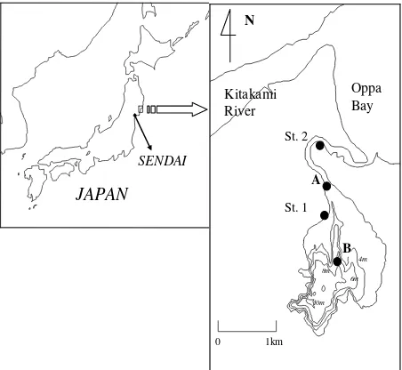
Period of simulation was 7 days in which the first day was a barotropic run up period. A period bet-ween two consecutive flood events of the Kitakami River, 2005/08/17-2005/05/24, was selected as simu-lation period during which the mid-layer intrusion mostly occurred due to buoyant enhanced strati-fication in the lagoon. During the simulation period, the wind continuously blew with minimum speed of 2.5 m/s. The longest extend of the main lagoon area is only around 3 km (see Fig. 2). Therefore, it was assumed that the resulting waves in the lagoon would never be in saturated condition due to the limited fetch condition. The waves were short, steep, and break more frequently and caused more turbulence near water surface.
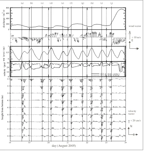
Fig. 3 shows, from top to bottom of the figure respectively, discharge at the Kitakami River, wind vector, water level and salinity that are used for open lateral boundary condition in all cases of simulation and flow velocity vectors of ADCP (Acoustic Doppler Current Profiler) measurement located at B (Fig. 2). The flow velocity was measured at the interval of 0.5 m, between 2 m and 6 m above the bottom. At the same location, three sensors of salinity and
temperature were also installed at distances of 3 m, 5 m from bottom, and 0.5 m from water surface. The flow velocity vectors show intermittence occurrence of mid-layer intrusion, which occur following high salinity flow into the lagoon. The effect of salinity to mid-layer intrusion is clearly shown in Fig. 3 at time marking (a) and (b). The time marking (a) shows higher salinity than (b) and consequently shows deeper intrusion, which is indicated by deeper occurrence of southward flow velocity vector. The lower salinity at (b) is caused by the East wind, which blown to the West. It is in agreement with the analysis shown by previous investigation [1]. Furthermore, the wind mostly occurred in the direction of East and West. In the figure, influence of the Kitakami River discharge is shown in the afternoon of August 23th, 2005. On that day, low salinity flowed to the lagoon following high discharge of the river. The figure shows also one distinctive characteristic of the lagoon entrance’s salinity in summer in which it has uniform vertical profile during flood tide and stratification state during ebb tide.
SENDAI
A
B
Figure 2. The Study Area
Calculations were carried out for three eddy viscosity/diffusivity parameterizations, which were constant eddy viscosity and diffusivity of 0.0005 m/s and 0.0 m/s respectively, QETE turbulence with conventional boundary condition, and QETE turbulence with wind enhanced breaking wave boundary condition. The suggested value of Craig
and Banner constant αCB of 100 was used for
breaking-wave enhanced turbulence kinetic energy calculation [16, 17, 22]. Additionally, supposedly waves in study area were young waves, surface
roughness length zs of 0.1 m was used in the
Results and Discussion
Eddy Viscosity and Eddy Diffusivity
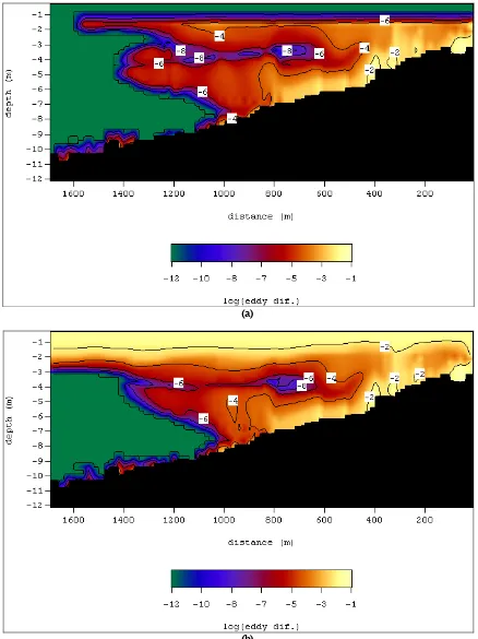
Figure 4(a) and Fig. 4(b) show eddy viscosity distributions, along the lagoon’s section passing from A then B (see Fig. 2) to inner lagoon, calculated using QETE turbulence model with conventional and breaking wave boundary condition respectively. Both figures correspond to time marking “h” in Fig.3. As expected, Fig. 4(b) shows higher eddy viscosity, which indicates higher mixing, near the surface up to depth of around 2.5 m. Below the depth, there is
no significant enhancement of eddy viscosity compared to Fig. 4(a). In addition, similar situations can be examined in Fig. 5(a) and Fig. 5(b), which show calculated eddy diffusivity using the QETE model with both types of the surface boundary conditions.
Vertical Profile of Velocity
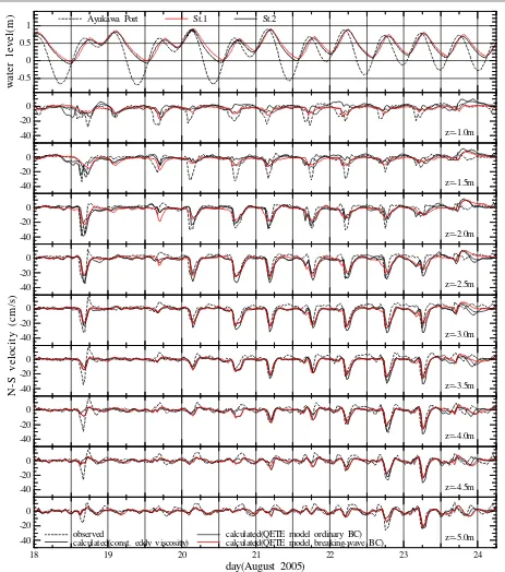
Time variations of observed and calculated
North-South velocity (UNS) are shown in Fig. 6. Similar
performance is obtained among the three cases of turbulent parameterization at depths starting from z=-2.0 m and lower. However, calculation using
0 0.5 1
wtr
l
e
v
e
l
(m)
0 1 0 2 0 3 0
sa
li
nit
y
(p
su
)
0 .5 m from surface 0 .5 m from b otto m (b) (c) (d) (e) (f) (g) (h) (i) (j)
day (August 2005)
= 20 cm/s = 10 m/s wind vector
velocity vector
N E
E N 0
200 400 600 800
di
sc
h
a
rg
e (
m
3 /s
)
h
eig
h
t fro
m
b
o
tt
o
m (m
)
(a)
constant eddy viscosity fails to reproduce the flow velocity at the two depths of z=-1.0 and z=-1.5. The other two calculations seem to give better agree-ments although they still result in underestimated
value. However, the parameterization of turbulence that includes breaking wave effect produces slight improvement of near surface velocities compared to the conventional one.
(a)
(b)
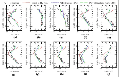
In addition to the time variation shown in Fig. 6, Fig. 7(a-j) shows vertical profiles of observed and
calculated UNS at selected representative time
during flood tides. Alphabetical numbering in the figure corresponds to time marking in Fig. 3. Dynamical equilibrium had probably not been achieved during the first day of baroclinic
calcu-lation. It is indicated by high discrepancies in Fig. 7(a). Although the observed and calculated profiles are in similar pattern, the constant eddy viscosity results in underestimated value near the surface. Moreover, inclusion of breaking-wave gives slight improvement of near surface flow velocity as indicated in (b), (c), (d), (f), (h), and (i) of Fig 7.
(a)
(b)
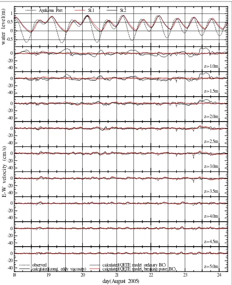
Figure 8 shows time variations of observed and
calculated East-West velocity (UEW). Basically, it is
observed that flow velocity in this direction is very small and the three calculations agree well with the observation. However, near the surface, the calcula-tion using constant eddy viscosity produces unrealis-tic currents at times of strong wind. The currents are in opposite direction of the wind, i.e. they are directed to the east when the east winds occur and, accordingly, they are directed to the west when the west winds blow. The currents are contributed from
unrealistic wind setup following the occurrence of strong wind. It seems that the constant eddy viscosity of 0.0005 m/s is not enough to produce turbulence viscosity. The viscosity must be higher at shallow regions located both on the east and the west sides of the dredged channel to prevent the rising of water level. The situations are less pronounced for the other turbulence parameterizations. Examinati-on to the figure shows that inclusiExaminati-on of breaking-wave effect produces the most realistic result. -0.5
0 0.5 1
w
a
te
r le
v
e
l(
m
) Ayukawa Port St.1 St.2
-40 -20 0
N
-S
v
e
lo
c
ity
(c
m
/s
)
z=-1.0m
-40 -20 0
z=-1.5m
-40 -20 0
z=-2.0m
-40 -20 0
z=-2.5m
-40 -20 0
z=-3.0m
-40 -20 0
z=-3.5m
-40 -20 0
z=-4.0m
-40 -20 0
z=-4.5m
18 19 20 21 22 23 24
day(August 2005)
-40 -20 0
z=-5.0m observed
calculated(const. eddy viscosity) calculated(QETE model ordinary BC) calculated(QETE model breaking-wave BC)
Conclusion
Simulation of density current in Nagatsura-ura Lagoon, Japan was carried out. Considering geometry shape of the study area and wind condition during numerical simulation, breaking wave enhanced turbulence kinetic energy was decided to be incorporated into the formulation of QETE turbulence closure by adopting Craig and Banner [17] surface boundary condition of turbulence kinetic energy equation. It is clear from simulation results that wind induced breaking-wave effect is quite significant. Simulation using Craig and Banner constant of 100 and surface roughness length of 0.1 m gives improvement to the resulted vertical profile of velocity, although still results in underestimate values near the water surface. The resulted eddy viscosity enhancement compared to the conventional boundary condition was found to occur near the surface up to depth of around 2.5 m.
Furthermore, although results of constant eddy viscosity parameterization is comparable to the other ones, it fails to reproduce the near surface flow velocities. The failure originates from its inability to produce sufficient mixing near the surface. In case of North-South flow velocity, the inability contributes to its low value near surface because of insufficient of turbulence viscosity to diffuse the velocity from
deeper layers. In case of East-West flow velocity, the lack of mixing contributes to its unrealistic value induced by unrealistic wind setup.
Near surface flow velocity can be important since it controls the movement of buoyant materials including fine suspended material brought into the lagoon during the flood tide. It affects spreading of the materials before their deposition. As the materials may contain rich nutrient, accurate prediction of their location of deposition is crucial since the nutrient will affect rate of oxygen consumption. It was found in this study that wind induced breaking-wave effect significantly influences near-surface profile of the mid-layer intrusion. Therefore, considering wind condition in the study area, breaking-wave effect on near surface flow velocity should be appropriately modeled as part of fine suspended particle and pollutant transport modeling.
Acknowledgements
The author would like to give his sincere gratitude to Professor Hitoshi Tanaka of Tohoku University for the data used in this research. Thanks must go to Susumu Kanayama, Dr. Eng. of Penta Ocean Technology for kindly providing well structured Fortran code of the three-dimensional hydrody-namics model and its very detail guidance.
-40 -20 0
UNS (cm/s)
2 4 6
h
e
ig
ht
f
rom
b
ot
to
m
(m
)
observed const. eddy vis. QETE(conv. BC) QETE(breaking-wave BC)
-40 -20 0
UNS(cm/s)
2 4 6
h
e
ig
ht
f
rom
b
ot
to
m
(m
)
-40 -20 0
UNS(cm/s)
2 4 6
h
e
ig
ht
fr
om
bot
tom
(
m
)
-40 -20 0
UN S(cm/s)
2 4 6
h
e
ig
ht
f
rom
b
ot
to
m
(m
)
-40 -20 0
UNS(cm/s)
2 4 6
h
e
ig
ht
f
rom
b
ot
to
m
(m
)
-40 -20 0
UN S(cm/s)
2 4 6
he
ig
ht
f
rom
b
ot
tom
(m
)
-40 -20 0
UNS(cm/s)
2 4 6
he
ig
ht
f
rom
b
ot
tom
(m
)
-40 -20 0
UNS(cm/s)
2 4 6
he
ig
ht
f
rom
b
ot
tom
(m
)
-40 -20 0
UN S(cm/s)
2 4 6
he
ig
ht
f
rom
b
ot
tom
(m
)
-40 -20 0
UNS(cm/s)
2 4 6
he
ig
ht
f
rom
b
ot
tom
(m
)
(a) (b) (c) (d) (e)
(f) (g) (h) (i) (j)
References
1. Okajima, N., Tanaka, H., Kanesato, M.,
Taka-saki, M., and Yamaji, H., Mechanism of DO
variation in Nagatsura-ura Lagoon, Proceedings
of Coastal Engineering JSCE, Vol.51, 2004, pp. 936-940 (in Japanese).
2. Rodi, W., Turbulence Models and Their
Applica-tion in Hydraulics, International Association for Hydraulic Research, Delft, Netherlands, 1980.
3. Rodi, W., Examples of calculation methods for
flow and mixing in stratified fluids, J. Geophys.
Res., 92, 1987, pp. 5305–5328.
-0.5 0 0.5 1
w
a
te
r l
e
v
e
l(
m
) Ayukawa Port St.1 St.2
-40 -20 0
E-W
ve
lo
c
it
y
(c
m
/s
)
z=-1.0m
-40 -20 0
z=-1.5m
-40 -20 0
z=-2.0m
-40 -20 0
z=-2.5m
-40 -20 0
z=-3.0m
-40 -20 0
z=-3.5m
-40 -20 0
z=-4.0m
-40 -20 0
z=-4.5m
18 19 20 21 22 23 24
day(August 2005)
-40 -20 0
z=-5.0m observed
calculated(const. eddy viscosity) calculated(QETE model ordinary BC) calculated(QETE model breaking-wave BC)
4. Mellor, G. L. and Yamada, T., Development of a turbulence closure model for geophysical fluid
problems, Rev. Geophys. Space Phys., 20, 1982,
pp. 851–875.
5. Burchard, H., Petersen, O., and Rippeth, T. P.,
Comparing the performance of the
Mellor-Yamada and the k-ε two-equation turbulence
models, J. Geogr. Res., 103, C5, 1998, pp.
10543-10554.
6. Burchard, H. and Petersen, O., Models of
turbu-lence in the marine environment- A comparative
study of two-equation turbulence models, J.
Marine Systems, 21, 1999, pp. 29-53.
7. Warner, J. C., Sherwood, C. R., Arango, H. G.,
Signell, R. P., and Butman, B., Performance of four turbulence closure methods implemented
with a generic length scale method, Ocean Model,
8, 2005, pp. 81– 113.
8. Warner, J. C., Geyer, W. R., and Lerczak, J. A.,
Numerical modeling of an estuary: A
comprehen-sive skill assessment, J. Geophys. Res., 110,
C05001, doi:10.1029/2004JC002691, 2005.
9. Li, M., Zhong, L., and Boicourt, W. C.,
Simula-tions of the Chesapeake Bay estuary: Sensitivity to turbulence mixing parameterisation and
comparison with observations, J. Geophys. Res.,
110, C12004, doi:10.1029/2004JC002585, 2005.
10.Wijesekera, H.W., Allen, J.S., and Newberger,
P.A., Modeling study of turbulent mixing over the continental shelf: comparison of turbulent closure
schemes, J. Geophys. Res., 108 (C3), 3103,
doi:10.1029/2001JC001234, 2003.
11.Durski, S. M., Glenn, S. M., and Haidvogel, D. B.,
Vertical mixing schemes in the coastal ocean: Comparison of the level 2.5 Mellor-Yamada scheme with an enhanced version of the K profile
parameterization, J. Geophys. Res., 109, C01015,
doi:10.1029/2002JC001702.2003JC001949, 2004.
12.Umlauf, L. and Burchard, H., A generic
length-scale equation for geophysical turbulence models,
J. Mar. Res., 61, 2003, pp. 235-265.
13.Galperin, B., Kantha, L. H., Hassid, S., and
Rosati, A., A quasi-equilibrium turbulent energy
model for geophysical flows, J. Atmos. Sci., 45,
1988, pp. 55-62.
14.Burchard, H., Simulating the wave-enhanced
layer under breaking surface waves with
two-equation turbulence models, J. Phys.Oceanogr.,
31, 2001, pp. 3133–3145.
15.Blumberg, A. F., Galperin, B., and O’Connor, D.
J., Modeling vertical structure of open-channel
flows, J. Hydr. Engrg., ASCE, 118(8), 1992, pp.
1119–1134.
16.Mellor, G. L. and Blumberg, A. F., Wave
Breaking and Ocean Surface Layer Thermal
Response, Journal of Physical Oceanography, 34,
2004, pp. 693-698.
17.Craig, P. D., and Banner M. L., Modeling
wave-enhanced turbulence in the ocean surface layer,
J. Phys. Oceanogr., 24, 1994, pp. 2546–2559.
18.Gross, E. S., Koseff, J. R., and Monismith, S. G.,
Three-dimensional salinity simulations of South
San Francisco Bay, J. Hydraul. Eng. ASCE,
125(11), 1999, pp. 1199–1209
19.Casulli, V. and Cheng, R. T., Semi-Implicit Finite
Difference Methods for Three-Dimensional
Shallow Water Flow, Int. Jour. for Numerical
Methods in Fluids, 15, 1992, pp. 629-648.
20.Purwanto, B. S., Study on flow and transport
mechanism in Nagatsura-ura lagoon, Sanriku Coast, Japan, Doctoral Dissertation, Tohoku University, Sendai, Japan, 2007.
21.Hoffman, J.D., Numerical Methods for Engineers
and Scientists, McGraw-Hill, New York, 1992.
22.Stacey, M. W. and Pond, S., On the Mellor–
Yamada turbulence closure scheme: The surface
boundary condition for q2, J. Phys. Oceanogr., 27,