A COMPARATIVE STUDY OF FORECASTING MODELS FOR
TREND AND SEASONAL TIME SERIES: DOES COMPLEX
MODEL ALWAYS YIELD BETTER FORECAST THAN SIMPLE
MODELS?
Suhartono
PhD Student, Mathematics Department, Gadjah Mada University, Yogyakarta, Indonesia e-mail: [email protected]
Subanar, Suryo Guritno
Mathematics Department, Gadjah Mada University, Yogyakarta, Indonesia e-mail: [email protected]
ABSTRACT
Many business and economic time series are non-stationary time series that contain trend and seasonal variations. Seasonality is a periodic and recurrent pattern caused by factors such as weather, holidays, or repeating promotions. A stochastic trend is often accompanied with the seasonal variations and can have a significant impact on various forecasting methods. In this paper, we will investigate and compare some forecasting methods for modeling time series with both trend and seasonal patterns. These methods are Winter’s, Decomposition, Time Series Regression, ARIMA and Neural Networks models. In this empirical research, we study on the effectiveness of the forecasting performance, particularly to answer whether a complex method always give a better forecast than a simpler method. We use a real data, that is airline passenger data. The result shows that the more complex model does not always yield a better result than a simpler one. Additionally, we also find the possibility to do further research especially the use of hybrid model by combining some forecasting method to get better forecast, for example combination between decomposition (as data preprocessing) and neural network model.
Keywords: Trend, seasonality, time series, Neural Networks, ARIMA, Decomposition, Winter’s, hybrid model.
1. INTRODUCTION
There are two basic considerations in producing an accurate and useful forecast. The first is to collect data that are relevant to the forecasting task and contain the information that can yield accurate forecast. The second key factor is to choose a forecasting technique that will utilize the information contained in the data and its pattern to the fulfilled.
Many business and economic time series are non-stationary time series that contain trend and seasonal variations. The trend is the long-term component that represents the growth or decline in the time series over an extended period of time. Seasonality is a periodic and recurrent pattern caused by factors such as weather, holidays, or repeating promotions. Accurate forecasting of trend and seasonal time series is very important for effective decisions in retail, marketing, production, inventory control, personnel, and many other business sectors (Makridakis and Wheelwright, 1987). Thus, how to model and forecast trend and seasonal time series has long been a major research topic that has significant practical implications.
and O’Connell, 1993; Hanke and Reitsch, 1995). Recently, Neural Networks (NN) models are also used for time series forecasting (see, for example, Hill et al., 1996; Faraway and Chatfield, 1998; Kaashoek and Van Dijk, 2001).
The purpose of this paper is to compare some forecasting models and to examine the issue whether a more complex model work more effectively in modeling and forecasting a trend and seasonal time series than a simpler model. In this research, NN model represents a more complex model, and other models (Winter’s, Decomposition, Time Series Regression and ARIMA) as a simpler model.
2. MODELING TREND AND SEASONAL TIME SERIES
Modeling trend and seasonal time series has been one of the main research endeavors for decades. In the early 1920s, the decomposition model along with seasonal adjustment was the major research focus due to Persons (1919, 1923) work on decomposing a seasonal time series. Holt (1957) and Winters (1960) developed method for forecasting trend and seasonal time series based on the weighted exponential smoothing. Among them, the work by Box and Jenkins (1976) on the seasonal ARIMA model has had a major impact on the practical applications to seasonal time series modeling. This model has performed well in many real world applications and is still one of the most widely used seasonal forecasting methods. More recently, NN have been widely used as a powerful alternative to traditional time series modeling (Zhang et al., 1998; Nelson et al., 1999; Hansen and Nelson, 2003). While their ability to model complex functional patterns in the data has been tested, their capability for modeling seasonal time series is not systematically investigated.
In this section, we will give a brief review of these forecasting models that usually used for forecasting a trend and seasonal time series.
2.1. Winter’s Exponential Smoothing
Exponential smoothing is a procedure for continually revising an estimate in the light of more recent experiences. Winter’s model is exponential smoothing model that usually used for forecasting trend and seasonal time series. The four equations used in Winter’s model are as follows (see Hanke and Reistch, 1995; page 172-173):
(i) The exponentially smoothed series:
1 1
(ii) The trend estimate:
β = smoothing constant for trend estimate (0< <β 1) γ = smoothing constant for seasonality estimate (0< <γ 1) L = length of seasonality.
2.2. Decomposition Method
In this section we present the multiplicative decomposition model. This model has been found to be useful when modeling time series that display increasing or decreasing seasonal variation (see Bowerman and O’Connell, 1993; chapter 7). The key assumption inherent in this model is that seasonality can be separated from other components of the series. The multiplicative decomposition model is
t t t t t
y = × × ×T S C I (5)
where
yt = the observed value of the time series in time period t
Tt = the trend component in time period t
St = the seasonal component in time period t
Ct = the cyclical component in time period t
It = the irregular component in time period t.
2.3. Time Series Regression
Time series regression models relate the dependent variable yt to functions of time. These
models are most profitably used when the parameters describing the time series to be forecast remain constant over time. For example, if a time series exhibits a linear trend, then the slope of the trend line remains constant. As another example, if the time series can be described by using monthly seasonal parameters, then the seasonal parameters for each of the twelve months remain the same from one year to the next. The time series regression model considered in this paper is (Bowerman and O’Connell, 1993; chapter 6):
t t t t
y = + +T S
ε
, (6)where
yt = the observed value of the time series in time period t
Tt = the trend in time period t
St = the seasonal factor in time period t
εt = the error term in time period t.
In this model, the seasonal factor is modeled by employing dummy variables.
2.4. Seasonal ARIMA Model
The seasonal ARIMA model belongs to a family of flexible linear time series models that can be used to model many different types of seasonal as well as nonseasonal time series. The seasonal ARIMA model can be expressed as (Cryer, 1986; Wei, 1990; Box et al., 1994):
( ) ( S)(1 ) (1d S)D ( ) ( S) p B P B B B yt q B Q B t
φ
Φ − − =θ
Θε
, (7)with
( ) p B
φ
= 1−φ
1B−φ
2B2− −…φ
pBp(
S)
P
B
( )
q
B
θ
=1
−
θ
1B
−
θ
2B
2− −
…
θ
qB
q(
S)
Q
B
Θ
=1
− Θ
1B
S− Θ
2B
2S− − Θ
…
QB
QS,where S is the seasonal length, B is the back shift operator and εt is a sequence of white noises with zero mean and constant variance. Box and Jenkins (1976) proposed a set of effective model building strategies for seasonal ARIMA based on the autocorrelation structures in a time series.
2.5. Neural Networks Model
Neural networks (NN) are a class of flexible nonlinear models that can discover patterns adaptively from the data. Theoretically, it has been shown that given an appropriate number of nonlinear processing units, NN can learn from experience and estimate any complex functional relationship with high accuracy. Empirically, numerous successful applications have established their role for pattern recognition and time series forecasting.
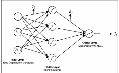
Feedforward Neural Networks (FFNN) is the most popular NN models for time series forecasting applications. Figure 1 shows a typical three-layer FFNN used for forecasting purposes. The input nodes are the previous lagged observations, while the output provides the forecast for the future values. Hidden nodes with appropriate nonlinear transfer functions are used to process the information received by the input nodes.
Figure 1. Architecture of Neural Network Model With Single Hidden Layer
The model of FFNN on Figure 1 can be written as
0
1 1
q p
t j ij t i oj t
j i
y
β
β
f
γ
y
−γ
ε
= =
= +
+
+
∑
∑
, (8)1 ( )
1 x
f x
e−
=
+ ’ (9)
{βj, j=0,1, , }q is a vector of weights from the hidden to output nodes and
{ ,γij i=0,1, , ;p j=1, 2, , }q are weights from the input to hidden nodes. Note that equation (8) indicates a linear transfer function is employed in the output node.
Functionally, the FFNN expressed in equation (8) is equivalent to a nonlinear AR model. This simple structure of the network model has been shown to be capable of approximating arbitrary function (Cybenko, 1989; Hornik et al., 1989, 1990; White, 1990). However, few practical guidelines exist for building a FFNN for a time series, particularly the specification of FFNN architecture in terms of the number of input and hidden nodes is not an easy task.
3. RESEARCH METHODOLOGY
The aim of this research is to provide empirical evidence on the comparative study of many forecasting models for modeling and forecasting trend and seasonal time series. The major research questions we investigate is:
Does the more complex model (FFNN) always yield a better forecast than the simpler model on forecasting trend and seasonal time series?
Is it possible to create hybrid model that combining some existing forecasting model for trend and seasonal time series?
To address these, we conduct empirical study with real data, the international airline passenger data. This data has been analyzed by many researchers, see for example Nam and Schaefer (1995), Hill et al. (1996), Faraway and Chatfield (1998), Atok and Suhartono (2000) and now become one of two data to be competed in Neural Network Forecasting Competition on June 2005 (see www.neural-forecasting.com).
3.1. Data
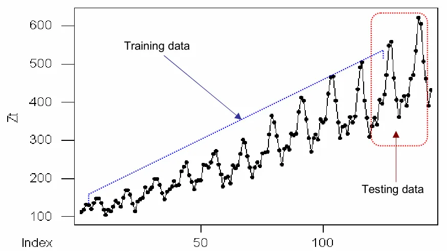
The international airline passenger data contain 144 month observations, started in January 1949 and ended in December 1960. The first 120 data observations are used for model selection and parameter estimation (training data in term of NN model) and the last 24 points are reserved as the test for forecasting evaluation and comparison (testing data). Figure 2 plots representative time series of this data. It is clear that the series has an upward trend together with seasonal variations.
3.2. Research Design
Specifically, Time Series Regression model building use logarithm transformation as data preprocessing to make seasonal variation become constant.
Figure 2. Time Series Plot of the International Airline Passenger Data
To determine the best FFNN architecture, an experiment is conducted with the basic cross validation method. The available training data is used to estimate the weights for any specific model architecture. The testing set is the used to select the best model among all models considered. In this study, the number of hidden nodes varies from 1 to 10 with an increment of 1. The lags of 1, 12 and 13 are included due to the results of Faraway and Chatfield (1998) and Atok and Suhartono (2000).
The FFNN model used in this empirical study is the standard FFNN with single-hidden-layer shown in Figure 1. We use S-Plus to conduct FFNN model building and evaluation. The initial value is set to random with 50 replications in each model to increase the chance of getting the global minimum. We also use data preprocessing by transform data to [-1,1] scale. The performance of in-sample fit and out-sample forecast is judged by three commonly used error measures. They are the mean squared error (MSE), the mean absolute error (MAE), and the mean absolute percentage error (MAPE).
4. EMPIRICAL RESULTS
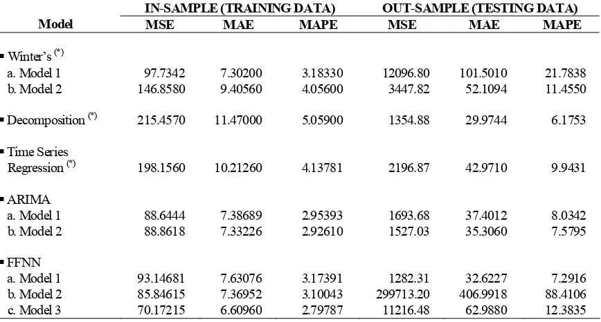
Table 1 summarizes the result of some forecasting models and reports performance measures across training and testing samples for the airline data. Several observations can be made from this table. First, decomposition method is a simple and useful model that yields a greater error measures than Winter’s, Time Series Regression and ARIMA model particularly in training data. On the other hand, this model gives a better (less) error measures in testing samples. Second, there are four ARIMA models that satisfied all criteria of good model and we present
two best of them on table 1. We can observe that the best ARIMA model in training set (model 1, ARIMA[0,1,1][0,1,1]12) yields worse forecast accuracy in testing samples than the second best ARIMA model (model 2, ARIMA[1,1,0][0,1,1]12). This result is exactly the same with Winter’s model, that is model 1 (α = 0.9, β =0.1 and γ =0.3) gives better forecast in training but worse result in testing than model 2 (α = 0.1, β =0.2 and γ =0.4).
Table 1. The Result of the Comparison Between Forecasting Models, Both in Training and Testing Data
IN-SAMPLE (TRAINING DATA) OUT-SAMPLE (TESTING DATA)
Model MSE MAE MAPE MSE MAE MAPE
: error model is not white noise
Third, the results of FFNN model have a similar trend. The more complex of FFNN architecture (it means the more number of unit nodes in hidden layer) always yields better result in training data, but the opposite result happened in testing sample. FFNN model 1, 2 and 3 respectively represent the number of unit nodes in hidden layer. We can clearly see that the more complex of FFNN model tends to overfitting the data in the training and due to have poor forecast in testing.
Finally, we also do diagnostic check in term of statistical modeling for each data to know especially whether the error model is white noise. From table 1 we know that Winter’s, Decomposition and Time series regression model do not yield the white noise errors. Only errors of ARIMA and FFNN models satisfied this condition. It means that modeling process of Winter’s, Decomposition and Time series regression are not finished and we can continue to model the errors by using other method. This condition give a chance to do further research by combining some forecasting method for trend and seasonal time series, for example combination between Time series regression and ARIMA (also known as combination deterministic-stochastic trend model), between Decomposition (as data preprocessing to make stationary data) and ARIMA, and also between Decomposition (as data preprocessing) and FFNN model.
5. CONCLUSIONS
Based on the results we can conclude that the more complex model does not always yield better forecast than the simpler one, especially on the testing samples. Our result only shows that the more complex FFNN model always yields better forecast in training data and it indicates an overfitting problem. Hence, the parsimonious FFNN model should be used in modeling and forecasting trend and seasonal time series.
Additionally, the results of this research also yield a chance to do further research on forecasting trend and seasonal time series by combining some forecasting methods, especially decomposition method as data preprocessing in NN model.
REFERENCES
Atok, R.M., Suhartono, 2000. “Comparison between Neural Networks, ARIMA Box-Jenkins and Exponential Smoothing Methods for Time Series Forecasting”, Research Report, Lemlit: Sepuluh Nopember Institute of Technology.
Box, G.E.P., G.M. Jenkins, 1976. Time Series Analysis: Forecasting and Control. San Fransisco: Holden-Day, Revised ed.
Box, G.E.P., G.M. Jenkins, G.C. Reinsel, 1994. Time Series Analysis, Forecasting and Control, 3rd ed, Englewood Cliffs: Prentice Hall.
Bowerman, B.L., O’Connel, 1993. Forecasting and Time Series: An Applied Approach, 3rd ed, Belmont, California: Duxbury Press.
Cryer, J.D., 1986. Time Series Analysis, Boston: PWS-KENT Publishing Company.
Cybenko, G., 1989. “Approximation by superpositions of a sigmoidal function”, Mathematics of
Control, Signals and Systems, 2, pp. 304–314.
Faraway, J., C. Chatfield, 1998. “Time series forecasting with neural network: a comparative study using the airline data”, Applied Statistics, 47, pp. 231–250.
Fildes, R., S. Makridakis, 1995. “The impact of empirical accuracy studies on time series analysis and forecasting”, International Statistical Review, 63 (3), pp. 289–308.
Hanke, J.E., A.G. Reitsch, 1995. Business Forecasting, Prentice Hall, Englewood Cliffs, NJ.
Hansen, J.V., R.D. Nelson, 2003. “Forecasting and recombining time-series components by using neural networks”, Journal of the Operational Research Society, 54 (3), pp. 307–317.
Hill, T., M. O’Connor, W. Remus, 1996. “Neural network models for time series forecasts”,
Management Science, 42, pp. 1082–1092.
Holt, C.C., 1957. “Forecasting seasonal and trends by exponentially weighted moving averages”,
Office of Naval Research, Memorandum No. 52.
Hornik, K., M. Stichcombe, H. White, 1989. “Universal approximation of an unknown mapping and its derivatives using multilayer feedforward networks”, Neural Networks, 3, pp. 551– 560.
Kaashoek, J. F., H. K. Van Dijk, 2001. Neural Networks as Econometric Tool, Report EI 2001– 05, Econometric Institute Erasmus University Rotterdam.
Makridakis, S., S.C. Wheelwright, 1987. The Handbook of Forecasting: A Manager’s Guide. 2nd Edition, John Wiley & Sons Inc., New York.
Nam, K., T. Schaefer, 1995. “Forecasting international airline passenger traffic using neural networks”, Logistics and Transportation Review, 31 (3), pp. 239–251.
Nelson, M., T. Hill, T. Remus, M. O’Connor, 1999. “Time series forecasting using NNs: Should the data be deseasonalized first?”, Journal of Forecasting, 18, pp. 359–367.
Persons, W.M., 1919. “Indices of business conditions”, Review of Economics and Statistics 1, pp. 5–107.
Persons, W.M., 1923. “Correlation of time series”. Journal of American Statistical Association, 18, pp. 5–107.
Wei, W.W.S., 1990. Time Series Analysis: Univariate and Multivariate Methods. Addison-Wesley Publishing Co., USA.
White, H., 1990. “Connectionist nonparametric regression: Multilayer feed forward networks can learn arbitrary mapping”, Neural Networks, 3, pp. 535–550.
Winters, P.R., 1960. “Forecasting Sales by Exponentially Weighted Moving Averages”,
Management Science, 6, pp. 324-342.