Introduction to
Electrical Engineering
Mulukutla S. Sarma
I N T R O D U C T I O N T O
the oxford series in electrical and computer engineering
Adel S. Sedra
, Series Editor
Allen and Holberg,
CMOS Analog Circuit Design
Bobrow,
Elementary Linear Circuit Analysis, 2nd Edition
Bobrow,
Fundamentals of Electrical Engineering, 2nd Edition
Burns and Roberts,
Introduction to Mixed Signal IC Test and Measurement
Campbell,
The Science and Engineering of Microelectronic Fabrication
Chen,
Analog & Digital Control System Design
Chen,
Digital Signal Processing
Chen,
Linear System Theory and Design, 3rd Edition
Chen,
System and Signal Analysis, 2nd Edition
DeCarlo and Lin,
Linear Circuit Analysis, 2nd Edition
Dimitrijev,
Understanding Semiconductor Devices
Fortney,
Principles of Electronics: Analog & Digital
Franco,
Electric Circuits Fundamentals
Granzow,
Digital Transmission Lines
Guru and Hiziro˘glu,
Electric Machinery and Transformers, 3rd Edition
Hoole and Hoole,
A Modern Short Course in Engineering Electromagnetics
Jones,
Introduction to Optical Fiber Communication Systems
Krein,
Elements of Power Electronics
Kuo,
Digital Control Systems, 3rd Edition
Lathi,
Modern Digital and Analog Communications Systems, 3rd Edition
Martin,
Digital Integrated Circuit Design
McGillem and Cooper,
Continuous and Discrete Signal and System Analysis, 3rd Edition
Miner,
Lines and Electromagnetic Fields for Engineers
Roberts and Sedra,
SPICE, 2nd Edition
Roulston,
An Introduction to the Physics of Semiconductor Devices
Sadiku,
Elements of Electromagnetics, 3rd Edition
Santina, Stubberud, and Hostetter,
Digital Control System Design, 2nd Edition
Sarma,
Introduction to Electrical Engineering
Schaumann and Van Valkenburg,
Design of Analog Filters
Schwarz,
Electromagnetics for Engineers
Schwarz and Oldham,
Electrical Engineering: An Introduction, 2nd Edition
Sedra and Smith,
Microelectronic Circuits, 4th Edition
Stefani, Savant, Shahian, and Hostetter,
Design of Feedback Control Systems, 3rd Edition
Van Valkenburg,
Analog Filter Design
Warner and Grung,
Semiconductor Device Electronics
Wolovich,
Automatic Control Systems
INTRODUCTION TO
ELECTRICAL ENGINEERING
Mulukutla S. Sarma
Northeastern University
New York
Oxford
Oxford University Press Oxford New York
Athens Auckland Bangkok Bogot´a Buenos Aires Calcutta
Cape Town Chennai Dar es Salaam Delhi Florence Hong Kong Istanbul Karachi Kuala Lumpur Madrid Melbourne Mexico City Mumbai
Nairobi Paris S˜ao Paulo Shanghai Singapore Taipei Tokyo Toronto Warsaw
and associated companies in Berlin Ibadan
Copyright © 2001 by Oxford University Press, Inc. Published by Oxford University Press, Inc.,
198 Madison Avenue, New York, New York, 10016 http://www.oup-usa.org
Oxford is a registered trademark of Oxford University Press
All rights reserved. No part of this publication may be reproduced, stored in a retrieval system, or transmitted, in any form or by any means, electronic, mechanical, photocopying, recording, or otherwise, without the prior permission of Oxford University Press.
Library of Congress Cataloging-in-Publication Data
Sarma, Mulukutla S., 1938–
Introduction to electrical engineering / Mulukutla S. Sarma
p. cm. — (The Oxford series in electrical and computer engineering) ISBN 0-19-513604-7 (cloth)
1. Electrical engineering. I. Title. II. Series. TK146.S18 2001
621.3—dc21 00-020033
Acknowledgments—Table 1.2.2 is adapted fromPrinciples of Electrical Engineering (McGraw-Hill Series in Electrical Engineering),by Peyton Z. Peebles Jr. and Tayeb A. Giuma, reprinted with the permission of McGraw-Hill, 1991; figures 2.6.1, 2.6.2 are adapted fromGetting Started with MATLAB 5: Quick Introduction,by Rudra Pratap, reprinted with the permission of Oxford University Press, 1998; figures 4.1.2–4.1.5, 4.2.1–4.2.3, 4.3.1–4.3.2, are adapted fromElectric Machines: Steady-State Theory and Dynamic Performance, Second Edition,by Mulukutla S. Sarma, reprinted with the permission of Brooks/Cole Publishing, 1994; figure 4.6.1 is adapted fromMedical Instrumentation Application and Design, by John G. Webster, reprinted with the permission of John Wiley & Sons, Inc., 1978; table 4.6.1 is adapted from “Electrical Safety in Industrial Plants,”IEEE Spectrum,by Ralph Lee, reprinted with the permission of IEEE, 1971; figure P5.3.1 is reprinted with the permission of Fairchild Semiconductor Corporation; figures 5.6.1, 6.6.1, 9.5.1 are adapted fromElectrical Engineering: Principles and Applications,by Allen R. Hambley, reprinted with the permission of Prentice Hall, 1997; figure 10.5.1 is adapted fromPower System Analysis and Design,Second Edition, by Duncan J. Glover and Mulukutla S. Sarma, reprinted with the permission of Brooks/Cole Publishing, 1994; figures 11.1.2, 13.2.10 are adapted fromIntroduction to Electrical Engineering, Second Edition,
by Clayton Paul, Syed A. Nasar, and Louis Unnewehr, reprinted with the permission of McGraw-Hill, 1992; figures E12.2.1(a,b), 12.2.2–12.2.5, 12.2.9– 12.2.10, 12.3.1–12.3.3, 12.4.1, E12.4.1, P12.1.2, P12.4.3, P12.4.8, P12.4.12, 13.1.1–13.1.8, 13.2.1–13.2.9, 13.2.11–13.2.16, 13.3.1–13.3.3, E13.3.2, 13.3.4, E13.3.3, 13.3.5–13.3.6 are adapted fromElectric Machines: Steady-State Theory and Dynamic Performance, Second Edition,by Mulukutla S. Sarma, reprinted with the permission of Brooks/Cole Publishing, 1994; figure 13.3.12 is adapted fromCommunication Systems Engineering,by John G. Proakis and Masoud Salehi, reprinted with the permission of Prentice Hall, 1994; figures 13.4.1–13.4.7, E13.4.1(b), 13.4.8–13.4.12, E13.4.3, 13.4.13, 13.6.1 are adapted fromElectric Machines: Steady-State Theory and Dynamic Performance, Second Edition,by Mulukutla S. Sarma Brooks/Cole Publishing, 1994; figures 14.2.8, 14.2.9 are adapted fromElectrical Engineering: Concepts and Applications, Second Edition, by A. Bruce Carlson and David Gisser, reprinted with the permission of Prentice Hall, 1990; figure 15.0.1 is adapted fromCommunication Systems, Third Edition,by A. Bruce Carlson, reprinted with the permission of McGraw-Hill, 1986; figures 15.2.15, 15.2.31, 15.3.11 are adapted fromCommunication Systems Engineering,
by John G. Proakis and Masoud Salehi, reprinted with the permission of Prentice Hall, 1994; figures 15.2.19, 15.2.27, 15.2.28, 15.2.30, 15.3.3, 15.3.4, 15.3.9, 15.3.10, 15.3.20 are adapted fromPrinciples of Electrical Engineering (McGraw-Hill Series in Electrical Engineering),by Peyton Z. Peebles Jr. and Tayeb A. Giuma, reprinted with the permission of McGraw-Hill, 1991; figures 16.1.1–16.1.3 are adapted fromElectric Machines: Steady-State Theory and Dynamic Performance, Second Edition,by Mulukutla S. Sarma, reprinted with the permission of Brooks/Cole Publishing, 1994; table 16.1.3 is adapted fromElectric Machines: Steady-State Theory and Dynamic Performance, Second Edition,by Mulukutla S. Sarma, reprinted with the permission of Brooks/Cole Publishing, 1994; table 16.1.4 is adapted fromHandbook of Electric Machines,by S. A. Nasar, reprinted with the permission of McGraw-Hill, 1987; and figures 16.1.4–13.1.9, E16.1.1, 16.1.10–16.1.25 are adapted fromElectric Machines: Steady-State Theory and Dynamic Performance, Second Edition,by Mulukutla S. Sarma, reprinted with the permission of Brooks/Cole Publishing, 1994.
Printing (last digit): 10 9 8 7 6 5 4 3 2 1
To my grandchildren
Puja Sree
Sruthi Lekha
Pallavi Devi
* * *
CONTENTS
List of Case Studies and Computer-Aided Analysis xiii
Preface xv
Overview xxi
PART 1
ELECTRIC CIRCUITS
1 Circuit Concepts
3
1.1 Electrical Quantities 4
1.2 Lumped-Circuit Elements 16
1.3 Kirchhoff’s Laws 39
1.4 Meters and Measurements 47
1.5 Analogy between Electrical and Other Nonelectric Physical Systems 50
1.6 Learning Objectives 52
1.7 Practical Application: A Case Study—Resistance Strain Gauge 52
Problems 53
2 Circuit Analysis Techniques
66
2.1 Thévenin and Norton Equivalent Circuits 66
2.2 Node-Voltage and Mesh-Current Analyses 71
2.3 Superposition and Linearity 81
2.4 Wye–Delta Transformation 83
2.5 Computer-Aided Circuit Analysis: SPICE 85
2.6 Computer-Aided Circuit Analysis: MATLAB 88
2.7 Learning Objectives 92
2.8 Practical Application: A Case Study—Jump Starting a Car 92
Problems 94
3 Time-Dependent Circuit Analysis
102
3.1 Sinusoidal Steady-State Phasor Analysis 103
3.2 Transients in Circuits 125
3.3 Laplace Transform 142
3.4 Frequency Response 154
viii CONTENTS
3.5 Computer-Aided Circuit Simulation for Transient Analysis, AC Analysis, and
Frequency Response Using PSpice and PROBE 168
3.6 Use of MATLAB in Computer-Aided Circuit Simulation 173
3.7 Learning Objectives 177
3.8 Practical Application: A Case Study—Automotive Ignition System 178
Problems 179
4 Three-Phase Circuits and Residential Wiring
198
4.1 Three-Phase Source Voltages and Phase Sequence 198
4.2 Balanced Three-Phase Loads 202
4.3 Measurement of Power 208
4.4 Residential Wiring and Safety Considerations 212
4.5 Learning Objectives 215
4.6 Practical Application: A Case Study—Physiological Effects of Current and Electrical Safety 216
Problems 218
PART 2
ELECTRONIC ANALOG AND DIGITAL SYSTEMS
5 Analog Building Blocks and Operational Amplifiers
223
5.1 The Amplifier Block 224
5.2 Ideal Operational Amplifier 229
5.3 Practical Properties of Operational Amplifiers 235
5.4 Applications of Operational Amplifiers 244
5.5 Learning Objectives 256
5.6 Practical Application: A Case Study—Automotive Power-Assisted Steering
System 257
Problems 258
6 Digital Building Blocks and Computer Systems
268
6.1 Digital Building Blocks 271
6.2 Digital System Components 295
6.3 Computer Systems 316
6.4 Computer Networks 320
6.5 Learning Objectives 325
6.6 Practical Application: A Case Study—Microcomputer-Controlled
Breadmaking Machine 325
Problems 326
7 Semiconductor Devices 339
7.1 Semiconductors 339
7.2 Diodes 340
CONTENTS ix
7.4 Field-Effect Transistors 367
7.5 Integrated Circuits 378
7.6 Learning Objectives 379
7.7 Practical Application: A Case Study—Electronic Photo Flash 380
Problems 380
8 Transistor Amplifiers
393
8.1 Biasing the BJT 394
8.2 Biasing the FET 395
8.3 BJT Amplifiers 399
8.4 FET Amplifiers 405
8.5 Frequency Response of Amplifiers 409
8.6 Learning Objectives 414
8.7 Practical Application: A Case Study—Mechatronics: Electronics Integrated
with Mechanical Systems 414
Problems 415
9 Digital Circuits 422
9.1 Transistor Switches 423
9.2 DTL and TTL Logic Circuits 427
9.3 CMOS and Other Logic Families 431
9.4 Learning Objectives 437
9.5 Practical Application: A Case Study—Cardiac Pacemaker, a Biomedical
Engineering Application 438
Problems 439
PART 3
ENERGY SYSTEMS
10
AC Power Systems
451
10.1 Introduction to Power Systems 452
10.2 Single- and Three-Phase Systems 455
10.3 Power Transmission and Distribution 460
10.4 Learning Objectives 466
10.5 Practical Application: A Case Study—The Great Blackout of 1965 466
Problems 468
11
Magnetic Circuits and Transformers 471
11.1 Magnetic Materials 472
11.2 Magnetic Circuits 475
11.3 Transformer Equivalent Circuits 479
11.4 Transformer Performance 486
11.5 Three-Phase Transformers 490
x CONTENTS
11.7 Learning Objectives 494
11.8 Practical Application: A Case Study—Magnetic Bearings for Space
Technology 494
Problems 495
12
Electromechanics 505
12.1 Basic Principles of Electromechanical Energy Conversion 505
12.2 EMF Produced by Windings 514
12.3 Rotating Magnetic Fields 522
12.4 Forces and Torques in Magnetic-Field Systems 526
12.5 Basic Aspects of Electromechanical Energy Converters 539
12.6 Learning Objectives 540
12.7 Practical Application: A Case Study—Sensors or Transducers 541
Problems 542
13
Rotating Machines 553
13.1 Elementary Concepts of Rotating Machines 553
13.2 Induction Machines 563
13.3 Synchronous Machines 582
13.4 Direct-Current Machines 594
13.5 Learning Objectives 610
13.6 Practical Application: A Case Study—Wind-Energy-Conversion
Systems 610
Problems 612
PART 4
INFORMATION SYSTEMS
14
Signal Processing 625
14.1 Signals and Spectral Analysis 626
14.2 Modulation, Sampling, and Multiplexing 640
14.3 Interference and Noise 649
14.4 Learning Objectives 658
14.5 Practical Application: A Case Study—Antinoise Systems, Noise
Cancellation 658
Problems 659
15
Communication Systems
666
15.1 Waves, Transmission Lines, Waveguides, and Antenna Fundamentals 670
15.2 Analog Communication Systems 685
15.3 Digital Communication Systems 710
15.4 Learning Objectives 730
15.5 Practical Application: A Case Study—Global Positioning Systems 731
CONTENTS xi
PART 5
CONTROL SYSTEMS
16
Basic Control Systems
747
16.1 Power Semiconductor-Controlled Drives 748
16.2 Feedback Control Systems 779
16.3 Digital Control Systems 805
16.4 Learning Objectives 814
16.5 Practical Application: A Case Study—Digital Process Control 815
Problems 816
Appendix A: References 831
Appendix B: Brief Review of Fundamentals of Engineering (FE) Examination 833
Appendix C: Technical Terms, Units, Constants, and Conversion Factors for the SI System 835
Appendix D: Mathematical Relations 838
Appendix E: Solution of Simultaneous Equations 843
Appendix F: Complex Numbers 846
Appendix G: Fourier Series 847
Appendix H: Laplace Transforms 851
LIST OF CASE STUDIES AND
COMPUTER-AIDED ANALYSIS
Case Studies
1.7 Practical Application: A Case Study—Resistance Strain Gauge 52 2.8 Practical Application: A Case Study—Jump Starting a Car 92
3.8 Practical Application: A Case Study—Automotive Ignition System 178
4.6 Practical Application: A Case Study—Physiological Effects of Current and Electrical Safety 216
5.6 Practical Application: A Case Study—Automotive Power-Assisted Steering System 257 6.6 Practical Application: A Case Study—Microcomputer-Controlled
Breadmaking Machine 325
7.7 Practical Application: A Case Study—Electronic Photo Flash 380
8.7 Practical Application: A Case Study—Mechatronics: Electronics Integrated with Mechanical
Systems 414
9.5 Practical Application: A Case Study—Cardiac Pacemaker, a Biomedical Engineering Application 438
10.5 Practical Application: A Case Study—The Great Blackout of 1965 466
11.8 Practical Application: A Case Study—Magnetic Bearings for Space Technology 494 12.7 Practical Application: A Case Study—Sensors or Transducers 541
13.6 Practical Application: A Case Study—Wind-Energy-Conversion Systems 610 14.5 Practical Application: A Case Study—Antinoise Systems, Noise Cancellation 658 15.5 Practical Application: A Case Study—Global Positioning Systems 731
16.5 Practical Application: A Case Study—Digital Process Control 815
Computer-Aided Analysis
2.5 Computer-Aided Circuit Analysis: SPICE 85 2.6 Computer-Aided Circuit Analysis: MATLAB 88
3.5 Computer-Aided Circuit Simulation for Transient Analysis, AC Analysis, and Frequency Response Using PSpice and PROBE 168
3.6 Use of MATLAB in Computer-Aided Circuit Simulation 173
PREFACE
I. OBJECTIVES
The purpose of this text is to present a problem-oriented introductory survey text for the ex-traordinarily interesting electrical engineering discipline by arousing student enthusiasm while addressing the underlying concepts and methods behind various applications ranging from con-sumer gadgets and biomedical electronics to sophisticated instrumentation systems, computers, and multifarious electric machinery. The focus is on acquainting students majoring in all branches of engineering and science, especially in courses fornonelectrical engineering majors, with the nature of the subject and the potentialities of its techniques, while emphasizing the principles. Since principles and concepts are most effectively taught by means of a problem-oriented course, judicially selected topics are treated in sufficient depth so as to permit the assignment of adequately challenging problems, which tend to implant the relevant principles in students’ minds.
In addition to an academic-year (two semesters or three quarters) introductory course traditionally offered to non-EE majors, the text is also suitable for a sophomore survey course given nowadays to electrical engineering majors in a number of universities. At a more rapid pace or through selectivity of topics, the introductory course could be offered in one semester to either electrical and computer engineering (ECE) or non-EE undergraduate majors. Although this book is written primarily for non-EE students, it is hoped that it will be of value to undergraduate ECE students (particularly for those who wish to take the Fundamentals of Engineering examination, which is a prerequisite for becoming licensed as a Professional Engineer), to graduate ECE students for their review in preparing for qualifying examinations, to meet the continuing-education needs of various professionals, and to serve as a reference text even after graduation.
II.
MOTIVATION
This text is but a modest attempt to provide an exciting survey of topics inherent to the electrical and computer engineering discipline. Modern technology demands a team approach in which electrical engineers and nonelectrical engineers have to work together sharing a common technical vocabulary. Nonelectrical engineers must be introduced to the language of electrical engineers, just as the electrical engineers have to be sensitized to the relevance of nonelectrical topics.
The dilemma of whether electrical engineering and computer engineering should be separate courses of study, leading to distinctive degrees, seems to be happily resolving itself in the direction of togetherness. After all, computers are not only pervasive tools for engineers but also their product; hence there is a pressing need to weave together the fundamentals of both the electrical and the computer engineering areas into the new curricula.
An almost total lack of contact between freshmen and sophomore students and the Department of Electrical and Computer Engineering, as well as little or no exposure to electrical and computer
xvi PREFACE
engineering, seems to drive even the academically gifted students away from the program. An initial spark that may have motivated them to pursue electrical and computer engineering has to be nurtured in the early stages of their university education, thereby providing an inspiration to continue.
This text is based on almost 40 years of experience teaching a wide variety of courses to electrical as well as non-EE majors and, more particularly, on the need to answer many of the questions raised by so many of my students. I have always enjoyed engineering (teaching, research, and consultation); I earnestly hope that the readers will have as much fun and excitement in using this book as I have had in developing it.
III.
PREREQUISITES AND BACKGROUND
The student will be assumed to have completed the basic college-level courses in algebra, trigonometry, basic physics, and elementary calculus. A knowledge of differential equations is helpful, but not mandatory. For a quick reference, some useful topics are included in the appendixes.
IV.
ORGANIZATION AND FLEXIBILITY
The text is developed to be student-oriented, comprehensive, and up to date on the subject with necessary and sufficient detailed explanation at the level for which it is intended. The key word in the organization of the text is flexibility.
The book is divided into five parts in order to provide flexibility in meeting different circumstances, needs, and desires. A glance at the Table of Contents will show that Part 1 concerns itself with basic electric circuits, in which circuit concepts, analysis techniques, time-dependent analysis including transients, as well as three-phase circuits are covered. Part 2 deals with electronic analog and digital systems, in which analog and digital building blocks are considered along with operational amplifiers, semiconductor devices, integrated circuits, and digital circuits. Part 3 is devoted to energy systems, in which ac power systems, magnetic circuits and transformers, principles of electromechanics, and rotating machines causing electromechanical energy conversion are presented. Part 4 deals with information systems, including the underlying principles of signal processing and communication systems. Finally, Part 5 presents control sys-tems, which include the concepts of feedback control, digital control, and power semiconductor-controlled drives.
The text material is organized for optimum flexibility, so that certain topics may be omitted without loss of continuity when lack of time or interest dictates.
V. FEATURES
PREFACE xvii
in basic concepts, a very wide range of engineering systems can be understood, analyzed, and devised.
3. The theory has been developed from simple beginnings in such a manner that it can readily be extended to new and more complicated situations. The art of reducing a practical device to an appropriate mathematical model and recognizing its limitations has been adequately presented. Sufficient motivation is provided for the student to develop interest in the analytical procedures to be applied and to realize that all models, being approximate representations of reality, should be no more complicated than necessary for the application at hand.
4. Since the essence of engineering is the design of products useful to society, the end objective of each phase of preparatory study should be to increase the student’s capability to design practical devices and systems to meet the needs of society. Toward that end, the student will be motivated to go through the sequence of understanding physical principles, processes, modeling, using analytical techniques, and, finally, designing.
5. Engineers habitually break systems up into their component blocks for ease of under-standing. The building-block approach has been emphasized, particularly in Part II concerning analog and digital systems. For a designer using IC blocks in assembling the desired systems, the primary concern lies with their terminal characteristics while the internal construction of the blocks is of only secondary importance.
6. Considering the world of electronics today, both analog and digital technologies are given appropriate coverage. Since students are naturally interested in such things as op amps, integrated circuits, and microprocessors, modern topics that can be of great use in their career are emphasized in this text, thereby motivating the students further.
7. The electrical engineering profession focuses on information and energy, which are the two critical commodities of any modern society. In order to bring the message to the forefront for the students’ attention, Parts III, IV, and V are dedicated to energy systems, information systems, and control systems, respectively. However, some of the material in Parts I and II is critical to the understanding of the latter.
An understanding of the principles of energy conversion, electric machines, and energy systems is important for all in order to solve the problems of energy, pollution, and poverty that face humanity today. It can be well argued that today’s non-EEs are more likely to encounter electromechanical machines than some of the ECEs. Thus, it becomes essential to have sufficient breadth and depth in the study of electric machines by the non-ECEs.
Information systems have been responsible for the spectacular achievements in communica-tion in recent decades. Concepts of control systems, which are not limited to any particular branch of engineering, are very useful to every engineer involved in the understanding of the dynamics of various types of systems.
8. Consistent with modern practice, the international (SI) system of units has been used throughout the text. In addition, a review of units, constants and conversion factors for the SI system can be found in Appendix C.
9. While solid-state electronics, automatic control, IC technology, and digital systems have become commonplace in the modern EE profession, some of the older, more traditional topics, such as electric machinery, power, and instrumentation, continue to form an integral part of the curriculum, as well as of the profession in real life. Due attention is accorded in this text to such topics as three-phase circuits and energy systems.
xviii PREFACE
11. Engineers who acquire a basic knowledge of electric circuits, electronic analog and digital circuits, energy systems, information systems, and control systems will have a well-rounded background and be better prepared to join a team effort in analyzing and designing systems. Therein lies the justification for the Table of Contents and the organization of this text.
12. At the end of each chapter, thelearning objectivesof that chapter are listed so that the student can check whether he or she has accomplished each of the goals.
13. At the very end of each chapter,Practical Application: A Case Studyhas been included so that the reader can get motivated and excited about the subject matter and its relevance to practice.
14. Basic material introduced in this book is totally independent of any software that may accompany the usage of this book, and/or the laboratory associated with the course. The common software in usage, as of writing this book, consists ofWindows, Word Perfect, PSPICE, Math CAD,andMATLAB. There are also other popular specialized simulation programs such asSignal Processing Workstation (SPW) in the area of analog and digital communications, Very High Level Description Language (VHDL)in the area of digital systems,Electromagnetic Transients Program (EMTP) in the field of power, and SIMULINK in the field of control. In practice, however, any combination of software that satisfies the need for word processing, graphics, editing, mathematical analysis, and analog as well as digital circuit analysis should be satisfactory.
In order to integrate computer-aided circuit analysis, two types of programs have been introduced in this text: A circuit simulator PSpice and a math solver MATLAB. Our purpose here is not to teach students how to use specific software packages, but to help them develop an analysis style that includes the intelligent use of computer tools. After all, these tools are an intrinsic part of the engineering environment, which can significantly enhance the student’s understanding of circuit phenomena.
15. The basics, to which the reader is exposed in this text, will help him or her to select consultants—experts in specific areas—either in or out of house, who will provide the knowledge to solve a confronted problem. After all, no one can be expected to be an expert in all areas discussed in this text!
VI.
PEDAGOGY
A. Outline
Beyond the overview meant as an orientation, the text is basically divided into five parts.
Part 1: Electric Circuits This part provides the basic circuit-analysis concepts and tech-niques that will be used throughout the subsequent parts of the text. Three-phase circuits have been introduced to develop the background needed for analyzing ac power systems. Basic notions of residential circuit wiring, including grounding and safety considerations, are presented.
Part 2: Electronic Analog and Digital Systems With the background of Part I, the student is then directed to analog and digital building blocks. Operational amplifiers are discussed as an especially important special case. After introducing digital system components, computer systems, and networks to the students, semiconductor devices, integrated circuits, transistor amplifiers, as well as digital circuits are presented. The discussion of device physics is kept to the necessary minimum, while emphasis is placed on obtaining powerful results from simple tools placed in students’ hands and minds.
PREFACE xix
Part 4: Information Systems Signal processing and communication systems (both analog and digital) are discussed using the block diagrams of systems engineering.
Part 5: Control Systems By focusing on control aspects, this part brings together the techniques and concepts of the previous parts in the design of systems to accomplish specific tasks. A section on power semiconductor-controlled drives is included in view of their recent importance. The basic concepts of feedback control systems are introduced, and finally the flavor of digital control systems is added.
Appendices The appendices provide ready-to-use information: Appendix A: Selected bibliography for supplementary reading
Appendix B: Brief review of fundamentals of engineering (FE) examination
Appendix C: Technical terms, units, constants, and conversion factors for the SI system Appendix D: Mathematical relations (used in the text)
Appendix E: Solution of simultaneous equations Appendix F: Complex numbers
Appendix G: Fourier series Appendix H: Laplace transforms
B. Chapter Introductions
Each chapter is introduced to the student stating the objective clearly, giving a sense of what to expect, and motivating the student with enough information to look forward to reading the chapter.
C. Chapter Endings
At the end of each chapter, thelearning objectivesof that chapter are listed so that the student can check whether he or she has accomplished each of the goals.
In order to motivate and excite the student, practical applications using electrical engineering principles are included. At the very end of each chapter, a relevantPractical Application: A Case Studyis presented.
D. Illustrations
A large number of illustrations support the subject matter with the intent to motivate the student to pursue the topics further.
E. Examples
Numerous comprehensive examples are worked out in detail in the text, covering most of the theoretical points raised. An appropriate difficulty is chosen and sufficient stimulation is built in to go on to more challenging situations.
F. End-of-Chapter Problems
A good number of problems (identified with each section of every chapter), with properly graded levels of difficulty, are included at the end of each chapter, thereby allowing the instructor considerable flexibility. There are nearly a thousand problems in the book.
G. Preparation for the FE Exam
A brief review of the Fundamentals of Engineering (FE) examination is presented in Appendix B in order to aid the student who is preparing to take the FE examination in view of becoming a registered Professional Engineer (PE).
VII. SUPPLEMENTS
xx PREFACE
MicroSoft PowerPoint Overheads to AccompanyIntroduction to Electrical Engineering (ISBN 019-514472-1) are free to adopters. Over 300 text figures and captions are available for classroom projection use.
Aweb-site,MSSARMA.org, will include interesting web links and enhancement materials, errata, a forum to communicate with the author, and more.
ACD-ROM Disk is packaged with each new book. The CD contains:
• Complete Solutions for Students to 20% of the problems.These solutions have been
prepared by the author and are resident on the disk in Adobe Acrobat (.pdf) format. The problems with solutions on disk are marked with an asterisk next to the problem in the text.
• The demonstration version of Electronics Workbench Multisim Version 6, an
in-novative teaching and learning software product that is used to build circuits and to simulate and analyze their electrical behavior. This demonstration version includes 20 demo circuit filesbuilt from circuit examples from this textbook. The CD also includes another80 circuitsfrom the text that can be opened with the full student or educational versions of Multisim. These full versions can be obtained from Electronics Workbench at www.electronicsworkbench.com.
To extend the introduction to selected topics and provide additional practice, we recommend the following additional items:
• Circuits:Allan’s Circuits Problemsby Allan Kraus (ISBN 019-514248-9), which includes
over 400 circuit analysis problems with complete solutions, many in MATLAB and SPICE form.
• Electronics:KC’s Problems and Solutions to Accompany Microelectronic Circuitsby K.C.
Smith (019–511771-9), which includes over 400 electronics problems and their complete solutions.
• SPICE:SPICEby Gordon Roberts and Adel Sedra (ISBN 019-510842-6) features over 100
examples and numerous exercises for computer-aided analysis of microelectronic circuits.
• MATLAB:Getting Started with MATLABby Rudra Pratap (ISBN 019-512947-4) provides
a quick introduction to using this powerful software tool.
For more information or to order an examination copy of the above mentioned supplements contact Oxford University Press at[email protected].
VIII.
ACKNOWLEDGMENTS
The author would like to thank the many people who helped bring this project to fruition. A number of reviewers greatly improved this text through their thoughtful comments and useful suggestions.
I am indebted to my editor, Peter C. Gordon, of Oxford University Press, who initiated this project and continued his support with skilled guidance, helpful suggestions, and great encouragement. The people at Oxford University Press, in particular, Senior Project Editor Karen Shapiro, have been most helpful in this undertaking. My sincere thanks are also due to Mrs. Sally Gupta, who did a superb job typing most of the manuscript.
I would also like to thank my wife, Savitri, for her continued encouragement and support, without which this project could not have been completed. It is with great pleasure and joy that I dedicate this work to my grandchildren.
OVERVIEW
What is electrical engineering? What is the scope of electrical engineering?
To answer the first question in a simple way, electrical engineering deals mainly with information systems and with power and energy systems. In the former, electrical means are used to transmit, store, and process information; while in the latter, bulk energy is transmitted from one place to another and power is converted from one form to another.
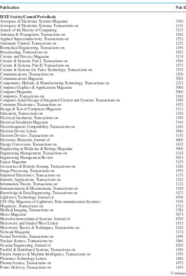
The second question is best answered by taking a look at the variety of periodicals published by the Institute of Electrical and Electronics Engineers (IEEE), which is the largest technical society in the world with over 320,000 members in more than 140 countries worldwide. Table I lists 75 IEEE Society/Council periodicals along with three broad-scope publications.
The transactions and journals of the IEEE may be classified into broad categories of devices, circuits, electronics, computers, systems, and interdisciplinary areas. All areas of electrical engineering require a working knowledge of physics and mathematics, as well as engineering methodologies and supporting skills in communications and human relations. A closely related field is that of computer science.
Obviously, one cannot deal with all aspects of all of these areas. Instead, the general concepts and techniques will be emphasized in order to provide the reader with the necessary background needed to pursue specific topics in more detail. The purpose of this text is to present the basic theory and practice of electrical engineering to students with varied backgrounds and interests. After all, electrical engineering rests upon a few major principles and subprinciples.
Some of the areas of major concern and activity in the present society, as of writing this book, are:
• Protecting the environment • Energy conservation • Alternative energy sources • Development of new materials • Biotechnology
• Improved communications
• Computer codes and networking
• Expert systems
This text is but a modest introduction to the exciting field of electrical engineering. However, it is the ardent hope and fervent desire of the author that the book will help inspire the reader to apply the basic principles presented here to many of the interdisciplinary challenges, some of which are mentioned above.
xxii OVERVIEW
TABLE I IEEE Publications
Publication Pub ID
IEEE Society/Council Periodicals
Aerospace & Electronic Systems Magazine 3161
Aerospace & Electronic Systems, Transactions on 1111
Annals of the History of Computing 3211
Antennas & Propagation, Transactions on 1041
Applied Superconductivity, Transactions on 1521
Automatic Control, Transactions on 1231
Biomedical Engineering, Transactions on 1191
Broadcasting, Transactions on 1011
Circuits and Devices Magazine 3131
Circuits & Systems, Part I, Transactions on 1561
Circuits & Systems, Part II, Transactions on 1571
Circuits & Systems for Video Technology, Transactions on 1531
Communications, Transactions on 1201
Communications Magazine 3021
Components, Hybrids, & Manufacturing Technology, Transactions on 1221
Computer Graphics & Applications Magazine 3061
Computer Magazine 3001
Computers, Transactions on 1161
Computer-Aided Design of Integrated Circuits and Systems, Transactions on 1391
Consumer Electronics, Transactions on 1021
Design & Test of Computers Magazine 3111
Education, Transactions on 1241
Electrical Insulation, Transactions on 1301
Electrical Insulation Magazine 3141
Electromagnetic Compatibility, Transactions on 1261
Electron Device Letters 3041
Electron Devices, Transactions on 1151
Electronic Materials, Journal of 4601
Energy Conversion, Transactions on 1421
Engineering in Medicine & Biology Magazine 3091
Engineering Management, Transactions on 1141
Engineering Management Review 3011
Expert Magazine 3151
Geoscience & Remote Sensing, Transactions on 1281
Image Processing, Transactions on 1551
Industrial Electronics, Transactions on 1131
Industry Applications, Transactions on 1321
Information Theory, Transactions on 1121
Instrumentation & Measurement, Transactions on 1101
Knowledge & Data Engineering, Transactions on 1471
Lightwave Technology, Journal of 4301
LTS (The Magazine of Lightwave Telecommunication Systems) 3191
Magnetics, Transactions on 1311
Medical Imaging, Transactions on 1381
Micro Magazine 3071
Microelectromechanical Systems, Journal of 4701
Microwave and Guided Wave Letters 1511
Microwave Theory & Techniques, Transactions on 1181
Network Magazine 3171
Neural Networks, Transactions on 1491
Nuclear Science, Transactions on 1061
Oceanic Engineering, Journal of 4201
Parallel & Distributed Systems, Transactions on 1501
Pattern Analysis & Machine Intelligence, Transactions on 1351
Photonics Technology Letters 1481
Plasma Science, Transactions on 1071
Power Delivery, Transactions on 1431
OVERVIEW xxiii
TABLE I Continued
Publication Pub ID
Power Electronics, Transactions on 4501
Power Engineering Review 3081
Power Systems, Transactions on 1441
Professional Communication, Transactions on 1251
Quantum Electronics, Journal of 1341
Reliability, Transactions on 1091
Robotics & Automation, Transactions on 1461
Selected Areas in Communication, Journal of 1411
Semiconductor Manufacturing, Transactions on 1451
Signal Processing, Transactions on 1001
Signal Processing Magazine 3101
Software Engineering, Transactions on 1171
Software Magazine 3121
Solid-State Circuits, Journal of 4101
Systems, Man, & Cybernetics, Transactions on 1271
Technology & Society Magazine 1401
Ultrasonics, Ferroelectrics & Frequency Control, Transactions on 1211
Vehicular Technology, Transactions on 1081
Broad Scope Publications
IEEE Spectrum 5001
Proceedings of the IEEE 5011
IEEE Potentials 5061
A historical perspective of electrical engineering, in chronological order, is furnished in Table II. A mere glance will thrill anyone, and give an idea of the ever-changing, fast-growing field of electrical engineering.
TABLE II Chronological Historical Perspective of Electrical Engineering
1750–1850 Coulomb’s law (1785) Battery discovery by Volta
Mathematical theories by Fourier and Laplace Ampere’s law (1825)
Ohm’s law (1827)
Faraday’s law of induction (1831)
1850–1900 Kirchhoff’s circuit laws (1857) Telegraphy: first transatlantic cables laid Maxwell’s equations (1864)
Cathode rays: Hittorf and Crookes (1869)
Telephony: first telephone exchange in New Haven, Connecticut
Edison opens first electric utility in New York City (1882): dc power systems Waterwheel-driven dc generator installed in Appleton, Wisconsin (1882) First transmission lines installed in Germany (1882), 2400 V dc, 59km Dc motor by Sprague (1884)
Commercially practical transformer by Stanley (1885) Steinmetz’s ac circuit analysis
Tesla’s papers on ac motors (1888) Radio waves: Hertz (1888)
First single-phase ac transmission line in United States (1889): Ac power systems, Oregon City to Portland, 4 kV, 21 km
First three-phase ac transmission line in Germany (1891), 12 kV, 179 km First three-phase ac transmission line in California (1893), 2.3 kV, 12 km Generators installed at Niagara Falls, New York
xxiv OVERVIEW
1900–1920 Marconi’s wireless telegraph system: transatlantic communication (1901) Photoelectric effect: Einstein (1904)
Vacuum-tube electronics: Fleming (1904), DeForest (1906) First AM broadcasting station in Pittsburgh, Pennsylvania Regenerative amplifier: Armstrong (1912)
1920–1940 Television: Farnsworth, Zworykin (1924)
Cathode-ray tubes by DuMont; experimental broadcasting Negative-feedback amplifier by Black (1927)
Boolean-algebra application to switching circuits by Shannon (1937)
1940–1950 Major advances in electronics (World War II) Radar and microwave systems: Watson-Watts (1940) Operational amplifiers in analog computers FM communication systems for military applications System theory papers by Bode, Shannon, and Wiener
ENIAC vacuum-tube digital computer at the University of Pennsylvania (1946) Transistor electronics: Shockley, Bardeen, and Brattain of Bell Labs (1947) Long-playing microgroove records (1948)
1950–1960 Transistor radios in mass production Solar cell: Pearson (1954)
Digital computers (UNIVAC I, IBM, Philco); Fortran programming language First commercial nuclear power plant at Shippingport, Pennsylvania (1957) Integrated circuits by Kilby of Texas Instruments (1958)
1960–1970 Microelectronics: Hoerni’s planar transistor from Fairchild Semiconductors Laser demonstrations by Maiman (1960)
First communications satelliteTelstar Ilaunched (1962) MOS transistor: Hofstein and Heiman (1963)
Digital communications
765 kV AC power lines constructed (1969) Microprocessor: Hoff (1969)
1970–1980 Microcomputers; MOS technology; Hewlett-Packard calculator INTEL’s 8080 microprocessor chip; semiconductor devices for memory Computer-aided design and manufacturing (CAD/CAM)
Interactive computer graphics; software engineering Personal computers; IBM PC
Artificial intelligence; robotics
Fiber optics; biomedical electronic instruments; power electronics
1980–Present Digital electronics; superconductors Neural networks; expert systems
I N T R O D U C T I O N T O
PART
1
Circuit Concepts
1.1 Electrical Quantities
1.2 Lumped-Circuit Elements
1.3 Kirchhoff’s Laws
1.4 Meters and Measurements
1.5 Analogy between Electrical and Other Nonelectric Physical Systems
1.6 Learning Objectives
1.7 Practical Application: A Case Study—Resistance Strain Gauge
Problems
Electric circuits, which are collections of circuit elements connected together, are the most fundamental structures of electrical engineering. A circuit is an interconnection of simple elec-trical devices that have at least one closed path in which current may flow. However, we may have to clarify to some of our readers what is meant by “current” and “electrical device,” a task that we shall undertake shortly. Circuits are important in electrical engineering because they process electrical signals, which carry energy and information; a signal can be any time-varying electrical quantity. Engineering circuit analysis is a mathematical study of some useful interconnection of simple electrical devices. An electric circuit, as discussed in this book, is
an idealized mathematical model of some physical circuit or phenomenon. The ideal circuit
elements are the resistor, the inductor, the capacitor, and the voltage and current sources. The ideal circuit model helps us topredict, mathematically, the approximate behavior of the actual event. The models also provide insights into how todesigna physical electric circuit to perform a desired task. Electrical engineering is concerned with theanalysisanddesignof electric circuits, systems, and devices. In Chapter 1 we shall deal with the fundamental concepts that underlie all circuits.
Electrical quantities will be introduced first. Then the reader is directed to the lumped-circuit elements. Then Ohm’s law and Kirchhoff’s laws are presented. These laws are sufficient
4 CIRCUIT CONCEPTS
for analyzing and designing simple but illustrative practical circuits. Later, a brief introduc-tion is given to meters and measurements. Finally, the analogy between electrical and other nonelectric physical systems is pointed out. The chapter ends with a case study of practical application.
1.1 ELECTRICAL QUANTITIES
In describing the operation of electric circuits, one should be familiar with such electrical quantities as charge, current, and voltage. The material of this section will serve as a review, since it will not be entirely new to most readers.
Charge and Electric Force
The proton has a charge of+1.602 10−19 coulombs (C), while the electron has a charge of −1.602×10⁻¹⁹ C. The neutron has zero charge. Electric charge and, more so, its movement are the most basic items of interest in electrical engineering. When many charged particles are collected together, larger charges and charge distributions occur. There may be point charges (C), line charges (C/m), surface charge distributions (C/m2), and volume charge distributions (C/m3).
A charge is responsible for an electric field and charges exertforces on each other. Like charges repel, whereas unlike charges attract. Such an electric force can be controlled and utilized for some useful purpose.Coulomb’s lawgives an expression to evaluate the electric force in newtons (N) exerted on one point charge by the other:
Force onQ1due toQ2 = ¯F21=
Q1Q2
4π ε0R2 ¯
a21 (1.1.1a)
Force onQ2due toQ1 = ¯F12=
Q2Q1
4π ε0R2 ¯
a12 (1.1.1b)
whereQ1andQ2are the point charges (C);Ris the separation in meters (m) between them;ε0
is the permittivity of the free-space medium with units of C2/N·m or, more commonly, farads
per meter (F/m); anda¯21anda¯12are unit vectors along the line joiningQ1andQ2, as shown in
Figure 1.1.1.
Equation (1.1.1) shows the following:
1. ForcesF¯21 andF¯12 are experienced byQ1 andQ2, due to the presence ofQ2andQ1,
respectively. They are equal in magnitude and opposite of each other in direction. 2. The magnitude of the force is proportional to the product of the charge magnitudes. 3. The magnitude of the force is inversely proportional to the square of the distance between
the charges.
4. The magnitude of the force depends on the medium.
5. The direction of the force is along the line joining the charges.
Note that the SI system of units will be used throughout this text, and the student should be conversant with the conversion factors for the SI system.
The force per unit charge experienced by a small test charge placed in an electric field is known as the electric field intensityE, whose units are given by N/C or, more commonly, volts¯ per meter (V/m),
¯
E= lim
Q→0
¯ F
1.1 ELECTRICAL QUANTITIES 5
R
Q1
Q2
a21
a12
F21
F12
Figure 1.1.1 Illustration of Coulomb’s law.
Equation (1.1.2) is the defining equation for the electric field intensity (with units of N/C or V/m), irrespective of the source of the electric field. One may then conclude:
¯
F21 =Q1E¯2 (1.1.3a)
¯
F12 =Q2E¯1 (1.1.3b)
whereE¯2is the electric field due toQ2 at the location ofQ1, andE¯1is the electric field due to
Q1at the location ofQ2, given by
¯ E2=
Q2
4π ε0R2 ¯
a21 (1.1.4a)
¯ E1=
Q1
4π ε0R2 ¯
a12 (1.1.4b)
Note that the electric field intensity due to a positive point charge is directed everywhere radially away from the point charge, and its constant-magnitude surfaces are spherical surfaces centered at the point charge.
EXAMPLE 1.1.1
(a) A small region of an impure silicon crystal with dimensions 1.25×10−6 m×10−3m
×10−3m has only the ions (with charge+1.6 10−19C) present with a volume density of 1025/m3. The rest of the crystal volume contains equal densities of electrons (with charge
−1.6×10⁻¹⁹C) and positive ions. Find the net total charge of the crystal.
(b) Consider the charge of part (a) as a point chargeQ1. Determine the force exerted by this
on a chargeQ2=3µC when the charges are separated by a distance of 2 m in free space,
as shown in Figure E1.1.1.
Q3 = −2 × 10⁻⁶ C
F12 F2 F32
Q2 = 3 × 10⁻⁶ C
2 m
1 m
76°
y
x Q1 = 2 × 10⁻⁶ C
−
+ +
6 CIRCUIT CONCEPTS
(c) If another chargeQ3= −2µC is added to the system 1 m aboveQ2, as shown in Figure
E1.1.1, calculate the force exerted onQ2.
S o l u t i o n
(a) In the region where both ions and free electrons exist, their opposite charges cancel, and the net charge density is zero. From the region containing ions only, the volume-charge density is given by
ρ=(1025)(1.6×10⁻¹⁹)=1.6×10⁶C/m3
The net total charge is then calculated as:
Q=ρv=(1.6×10⁶)(1.25×10−6×10−3×10⁻³)=2×10⁻⁶C
(b) The rectangular coordinate system shown defines the locations of the charges: Q1 =
2×10⁻⁶C;Q
2=3×10⁻⁶C. The force thatQ1exerts onQ2is in the positive direction
ofx, given by Equation (1.1.1),
¯ F12=
(3×10⁻⁶)(2×10⁻⁶)
4π(10−9/36π )22 a¯x = ¯ax13.5×10
−3N
This is the force experienced byQ2due to the effect of the electric field ofQ1. Note the
value used for free-space permittivity,ε0, as (8.854×10⁻¹²), or approximately 10−9/36π
F/m.a¯x is the unit vector in the positivex-direction.
(c) WhenQ3is added to the system, as shown in Figure E1.1.1, an additional force onQ2
directed in the positivey-direction occurs (sinceQ3andQ2are of opposite sign),
¯ F32=
(3×10⁻⁶)(−2×10⁻⁶)
4π(10−936π )12 (− ¯ay)= ¯ay54×10
−3 N
The resultant forceF¯2acting onQ2 is the superposition ofF¯12andF¯32due toQ1and
Q3, respectively.
The vector combination ofF¯12andF¯32is given by:
¯ F2=
F122 +F322 tan−1F¯32
¯ F12
=13.52+542×10−3 tan−1 54
13.5
=55.7×10⁻³ 76° N
Conductors and Insulators
1.1 ELECTRICAL QUANTITIES 7
Insulatorsare materials that do not allow charge to move easily. Examples include glass, plastic, ceramics, and rubber. Electric current cannot be made to flow through an insulator, since a charge has great difficulty moving through it. One sees insulating (ordielectric) materials often wrapped around the center conducting core of a wire.
Although the term resistance will be formally defined later, one can say qualitatively that a conductor has a very low resistance to the flow of charge, whereas an insulator has a very high resistance to the flow of charge. Charge-conducting abilities of various materials vary in a wide range.Semiconductors fall in the middle between conductors and insulators, and have a moderate resistance to the flow of charge. Examples include silicon, germanium, and gallium arsenide.
Current and Magnetic Force
The rate of movement of net positive charge per unit of time through a cross section of a conductor is known ascurrent,
i(t )=dq
dt (1.1.5)
The SI unit of current is the ampere (A), which represents 1 coulomb per second. In most metallic conductors, such as copper wires, current is exclusively the movement of free electrons in the wire. Since electrons are negative, and since the direction designated for the current is that of the net positive charge movement, the charges in the wire are thus moving in the direction opposite to the direction of the current designation. The net charge transferred at a particular time is the net area under the current–time curve from the beginning of time to the present,
q(t )= t
−∞
i(τ ) dτ (1.1.6)
While Coulomb’s law has to do with the electric force associated with two charged bodies, Ampere’s law of forceis concerned with magnetic forces associated with two loops of wire carrying currents by virtue of the motion of charges in the loops. Note that isolated current elements do not exist without sources and sinks of charges at their ends; magnetic monopoles do not exist. Figure 1.1.2 shows two loops of wire in freespace carrying currentsI1andI2.
Considering a differential elementdl¯1 of loop 1 and a differential elementdl¯2 of loop 2,
the differential magnetic forcesdF¯21anddF¯12 experienced by the differential current elements
I1dl¯1, andI2dl¯2, due toI2andI1, respectively, are given by
dF¯21=I1dl¯1×
µ
0
4π
I2dl¯2× ¯a21
R2
(1.1.7a)
dF¯12=I2dl¯2×
µ0
4π
I1dl¯1× ¯a12
R2
(1.1.7b)
wherea¯21anda¯12are unit vectors along the line joining the two current elements,Ris the distance
between the centers of the elements,µ0 is the permeability of free space with units of N/A2or
commonly known as henrys per meter (H/m). Equation (1.1.7) reveals the following:
8 CIRCUIT CONCEPTS
Loop 1 Loop 2
R I1 I2
a12 dl1
dl2 a21
Figure 1.1.2 Illustration of Ampere’s law (of force).
2. The magnitude of the force is inversely proportional to the square of the distance between the current elements.
3. To determine the direction of, say, the force acting on the current elementI1dl¯1, thecross
productdl¯2× ¯a21 must be found. Then crossingdl¯1 with the resulting vector will yield
the direction ofdF¯21.
4. Each current element is acted upon by amagnetic fielddue to the other current element,
dF¯21=I1dl¯1× ¯B2 (1.1.8a)
dF¯12=I2dl¯2× ¯B1 (1.1.8b)
whereB¯ is known as themagnetic flux density vectorwith units of N/A·m, commonly known as webers per square meter (Wb/m2) or tesla (T).
Current distribution is the source of magnetic field, just as charge distribution is the source of electric field. As a consequence of Equations (1.1.7) and (1.1.8), it can be seen that
¯ B2=
µ0
4π I2dl¯2× ¯a21 (1.1.9a)
¯ B1=
µ0
4π
I1dl¯1× ¯a12
R2 (1.1.9b)
which depend on the medium parameter. Equation (1.1.9) is known as theBiot–Savart law.
Equation (1.1.8) can be expressed in terms of moving charge, since current is due to the flow of charges. WithI = dq/dt anddl¯= ¯v dt, wherev¯ is the velocity, Equation (1.1.8) can be rewritten as
dF¯ =
dq dt
(v dt )¯ × ¯B=dq (v¯× ¯B) (1.1.10)
Thus it follows that the forceF¯ experienced by a test charge q moving with a velocityv¯ in a magnetic field of flux densityB¯ is given by
¯
F =q (v¯× ¯B) (1.1.11)
The expression for the total force acting on a test chargeq moving with velocityv¯in a region characterized by electric field intensityE¯ and a magnetic field of flux densityB¯is
¯
F = ¯FE+ ¯FM =q (E¯+ ¯v× ¯B) (1.1.12)
1.1 ELECTRICAL QUANTITIES 9
EXAMPLE 1.1.2
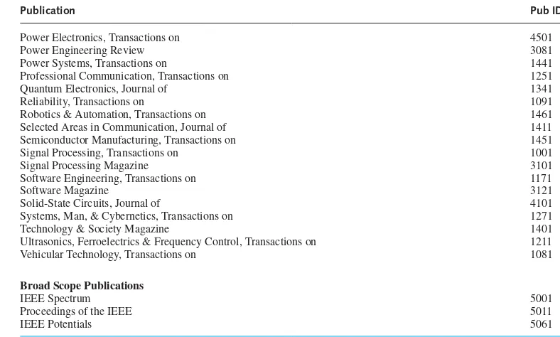
Figure E1.1.2 (a) gives a plot ofq(t )as a function of timet.
(a) Obtain the plot ofi(t ).
(b) Find the average value of the current over the time interval of 1 to 7 seconds.
3
t, seconds
−1
0 1 2 3 4 5 6 7 8 9 10
q(t), coulombs
(a)
t, seconds
i(t), amperes
−2.0
(b) 1.0 1.5
1 2 3 4 5 6 7 8 9 10
Figure E1.1.2 (a) Plot of q(t ).
(b)Plot ofi(t ).
S o l u t i o n
(a) Applying Equation (1.1.5) and interpreting the first derivative as the slope, one obtains the plot shown in Figure E1.1.2(b).
(b) Iav =(1/T )
T
0 i dt. Interpreting the integral as the area enclosed under the curve, one
gets:
Iav= 1
(7−1)[(1.5×2)−(2.0×2)+(0×1)+(1×1)]=0
10 CIRCUIT CONCEPTS
EXAMPLE 1.1.3
Consider an infinitesimal length of 10−6m of wire whose center is located at the point (1, 0, 0),
carrying a current of 2 A in the positive direction ofx.
(a) Find the magnetic flux density due to the current element at the point (0, 2, 2).
(b) Let another current element (of length 10−3m) be located at the point (0, 2, 2), carrying a current of 1 A in the direction of(− ¯ay+ ¯az). Evaluate the force on this current element due to the other element located at (1, 0, 0).
S o l u t i o n
(a) I1dl¯1=2×10⁻⁶a¯x. The unit vectora¯12is given by
¯ a12=
(0−1)a¯x+(2−0)a¯y+(2−0)a¯z
√
12+22+22
= (− ¯ax+2a¯y+2a¯z)
3
Using the Biot–Savart law, Equation (1.1.9), one gets
[B¯1](0,2,2)=
µ0
4π
I1dl¯1× ¯a12
R2
whereµ0is the free-space permeability constant given in SI units as 4π ×10−7 H/m,
andR2in this case is{(0−1)2+(2−0)2+(2−0)2}, or 9. Hence,
[B¯1](0,2,2)=
4π×10−7 4π
(2×10⁻⁶a¯x)×(− ¯ax+2a¯y+2a¯z) 9×3
= 10
−7
27 ×4×10 −6(
¯
az− ¯ay)Wb/m2
=0.15×10⁻¹³(a¯z− ¯ay)T (b) I2dl¯2=10−3(− ¯ay+ ¯az)
dF¯12 =I2dl¯2× ¯B1
= 10−3(− ¯ay+ ¯az)
× 0.15×10⁻¹³(a¯z− ¯ay)
=0
Note that the force is zero since the current elementI2dl¯2and the fieldB¯1due toI1dl¯1
at (0, 2, 2) are in the same direction.
The Biot–Savart law can be extended to find the magnetic flux density due to a current-carrying filamentary wire of any length and shape by dividing the wire into a number of infinitesimal elements and using superposition. The net force experienced by a current loop can be similarly evaluated by superposition.
Electric Potential and Voltage
1.1 ELECTRICAL QUANTITIES 11
v(x)= dw(x)
dq (1.1.13)
where w(x)is the potential energy that a particle with chargeq has when it is located at the positionx. The zero point of potential energy can be chosen arbitrarily since only differences in energy have practical meaning. The point where electric potential is zero is known as thereference pointor ground point, with respect to which potentials at other points are then described. The potential differenceis known as thevoltageexpressed in volts (V) or joules per coulomb (J/C). If the potential atBis higher than that atA,
vBA=vB−vA (1.1.14)
which is positive. Obviously voltages can be either positive or negative numbers, and it follows that
vBA= −vAB (1.1.15)
The voltage at point A, designated asvA, is then the potential at point A with respect to the ground.
Energy and Power
If a chargedqgives up energydwwhen going from pointato pointb, then the voltage across those points is defined as
v= dw
dq (1.1.16)
Ifdw/dq is positive, pointa is at the higher potential. The voltage between two points is the work per unit positive charge required to move that charge between the two points. Ifdwanddq have the same sign, then energy isdeliveredby a positive charge going fromatob(or a negative charge going the other way). Conversely, charged particlesgainenergy inside asourcewheredw anddqhave opposite polarities.
The load and source conventions are shown in Figure 1.1.3, in which point a is at a higher potential than point b. The loadreceives or absorbs energy because a positive charge goes in the direction of the current arrow from higher to lower potential. The source has
a capacity to supply energy. The voltage source is sometimes known as an electromotive
force, or emf, to convey the notation that it is a force that drives the current through the circuit.
The instantaneous power pis defined as the rate of doing work or the rate of change of energydw/dt,
p=dw
dt =
dw
dq dq dt
=vi (1.1.17)
The electric power consumed or produced by a circuit element is given by its voltage–current product, expressed in volt-amperes (VA) or watts (W). The energy over a time interval is found by integrating power,
w=
T
0
p dt (1.1.18)
12 CIRCUIT CONCEPTS
Load iab
vab
a
b
+
−
Source iba
vab
a
i
b
+
−
Figure 1.1.3 Load and source conventions.
EXAMPLE 1.1.4
A typical 12-V automobile battery, storing about 5 megajoules (MJ) of energy, is connected to a 4-A headlight system.
(a) Find the power delivered to the headlight system. (b) Calculate the energy consumed in 1 hour of operation.
(c) Express the auto-battery capacity in ampere-hours (Ah) and compute how long the headlight system can be operated before the battery is completely discharged.
S o l u t i o n
(a) Power delivered:P =V I =124=48W.
(b) AssumingVandIremain constant, the energy consumed in 1 hour will equal
W =48(60×60)=172.8×10³J=172.8kJ
(c) 1 Ah = (1 C/s)(3600 s) = 3600C. For the battery in question, 5×10⁶J/12 V =
0.417×10⁶C. Thus the auto-battery capacity is 0.417×10⁶/3600∼
=116 Ah. Without completely discharging the battery, the headlight system can be operated for 116/4=29 hours.
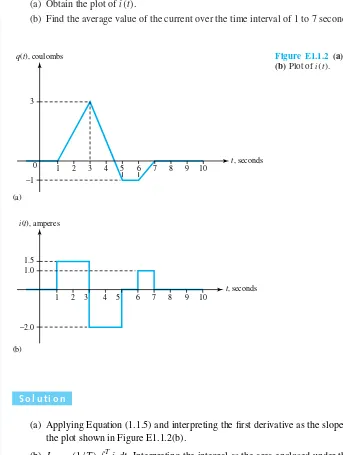
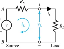
Sources and Loads
A source–load combination is represented in Figure 1.1.4. Anodeis a point at which two or more components or devices are connected together. A part of a circuit containing only one component, source, or device between two nodes is known as abranch. A voltageriseindicates an electric source, with the charge being raised to a higher potential, whereas a voltagedrop indicates a load, with a charge going to a lower potential. The voltageacrossthe source is the same as the voltage across the load in Figure 1.1.4. The current delivered by the source goes throughthe load. Ideally, with no losses, the power(p=vi)delivered by the source is consumed by the load.