VOXEL BASED SEGMENTATION OF LARGE AIRBORNE TOPOBATHYMETRIC
LIDAR DATA
R. Boerner,∗, L. Hoegner, U. Stilla
Photogrammetry and Remote Sensing, Technical University of Munich 80333 Munich, Germany - (richard.boerner, ludwig.hoegner, stilla)@tum.de
Commission II, WG II/3
KEY WORDS:Point cloud, large-scale dataset, Segmentation, Classification, Ground extraction, Voxel structure
ABSTRACT:
Point cloud segmentation and classification is currently a research highlight. Methods in this field create labelled data, where each point has additional class information. Current approaches are to generate a graph on the basis of all points in the point cloud, calculate or learn descriptors and train a matcher for the descriptor to the corresponding classes. Since these approaches need to look on each point in the point cloud iteratively, they result in long calculation times for large point clouds. Therefore, large point clouds need a generalization, to save computation time. One kind of generalization is to cluster the raw points into a 3D grid structure, which is represented by small volume units ( i.e. voxels) used for further processing. This paper introduces a method to use such a voxel structure to cluster a large point cloud into ground and non-ground points. The proposed method for ground detection first marks ground voxels with a region growing approach. In a second step non ground voxels are searched and filtered in the ground segment to reduce effects of over-segmentations. This filter uses the probability that a voxel mostly consist of last pulses and a discrete gradient in a local neighbourhood . The result is the ground label as a first classification result and connected segments of non-ground points. The test area of the river Mangfall in Bavaria, Germany, is used for the first processing.
1. INTRODUCTION
The European directive forces the creation of change maps of river areas (European Union, 2000, 2007). To create these maps, the cheapest and fastest way is to use airborne LiDAR with a green laser. This technique measures a set of points mapping the water surface, river ground and the river waterfront. Such a set of points is called topobathymetric point cloud. Creating change maps of river areas needs a change detection of topobathymetric point clouds which determines missing or new areas between two times (e.g. caused by depositions or drifts of the river ground). To implement such a change detection on the basis of topobathy-metric point clouds, the first step is a segmentation and classifica-tion. Class labels like building, vegetation, water, wet ground and dry ground will be used for the change detection task by defining thresholds for a change significance. For example, the ground under the water surface (i. e. wet ground) changes with a higher probability as the dry ground, because of the river’s morphody-namic. Furthermore, the most important classes for the analy-sis of topobathymetric point clouds are water and ground. The water class must be known to correct the influence of different light refraction characteristics of water and air (Mandlburger et al., 2015).
A first classification is achieved by a segmentation of the point cloud into ground and non-ground points. Such ground detection approaches use a region growing which is computational expen-sive in the case of a huge number of points in the scanned data. To save computation time, it is necessary to generalize the point cloud which can be done with a structure of volume clusters. These so called voxels generalize the point cloud by summariz-ing points, which are inside the same volume part. The proposed segmentation uses a region growing approach on the basis of a
∗Corresponding author
voxel structure. This method is able to process large-scale air-borne LiDAR data with the aim of creating segments like ground and non ground. The focus of the approach is a fast computation even if the point cloud data becomes large. The voxel structure, used for this approach, is generated with an octree and the time consumed for the computation depends only on the size of the initial bounding box. Therefore the computation cost is almost independent of the number of points in the point cloud.
This paper is structured as follows: Section 2 will sparsely review some state of the art approaches of the topic point cloud segmen-tation and classification. Section 3 will introduces the proposed method and explain how to use it for ground detection and seg-mentation tasks. The used data will be illustrated and character-ized in section 4. Afterwards, section 5 shows first results of the proposed approach and the used data, which is introduced before. At the end, section 6 gives a short summary.
2. RELATED WORK
The classification task can be divided into two major parts: the segmentation and the use of these segments for a matching of class labels. The aim of the segmentation is to create regions of connected points. Most state of the art approaches are point based approaches. That means each point of the point cloud needs to be processed. Such point based segmentation approaches can be find in Rutzinger et al. (2008); Shapovalov et al. (2010); Zhang et al. (2016).
Zhang et al. (2016) build an undirected graph of each non terrain point to its k-nearest neighbours. To create segments on the ba-sis of this graph, they determine the local maxima of the points height value and perform a graph cut at this local maxima. This graph cut clusters the whole graph into smaller parts, which are normalized by a predefined threshold for the number of points of each segment.
Shapovalov et al. (2010) use a machine learning approach to get the class labels for each point. A Markov random field is used to build a graph on the base of all points. The connection of nodes in the graph is determined by unary and pairwise potentials. The unary potential can be seen as the descriptor for a single point and the pairwise potential as the descriptor for an edge in the graph. Shapovalov et al. (2010) use for the unary potential spectral and directional features, spin images, angular spin images and distri-butions of heights. Their pairwise potential depends on the angle between normals, the difference in altitudes and the difference in positions of two neighboured points. The unary potential is computed with a random forest classifier and the pairwise poten-tial with the Na¨ıve Bayes classifier. The final class label for each point is identified with the Markov random field inference
A similar approach, adopting conditional random fields for point cloud classification, is propsed by Niemeyer et al. (2014). They obtain the unary and pairwise potential with linear models trained with the random forest algorithm. These models use a long list of attributes like intensity, echo numbers, height of a single point above DTM, residuals from a local plane fitting, and others.
Zhang et al. (2016) train SCLDA-based features for their point wise descriptors and match these descriptors to a class label with the AdaBoost classifier. Reitberger et al. (2009) show how to segment point clouds into tree crown and tree stem segments by using a graph cut approach.
Previous work for segmentation uses a modelling of the geom-etry sampled with a voxel structure (Xu et al., 2017). This pa-per introduces a graph based segmentation of a local fully con-nected affinity graph. Instead of a pair of voxels the used affinity graph considers all voxels in the local neighourhood. Inside this graph, voxels are connected in dependence on their spatial dis-tance, shape similarity and surface connectivity corresponding to smoothness and convexity criterions. This method shows suitable results for segmentation of building elements by recognizing ge-ometric primitives. Furthermore, a supervoxel approach for seg-mentation of outdoor scenes is shown in Xu et al. (2016). This uses a connection judgement dependent on eigenvalue based ge-ometric features. This features are used to calculate similarities between two voxels. This approach also creates good results for clustering point clouds into geometric primitives, but also shows difficulties in case of vegetation. Unfortunately, large scale air-borne LIDAR data is drawn by few geometric elements (i.e. only buildings and flat ground parts can be modelled with geometric primitives). Therefore, further development is needed for dealing with non urban areas.
Aijazi et al. (2013) combine voxels to one segment if the voxels are close in position and their intensity- or colour differences are lower than a predefined threshold. To match the voxel segments to a class label, they use the surface normal, the height difference between geometrical - and barycentre, geometrical shape, color, and intensity.
The proposed approach in this paper is based on this voxel seg-mentation used by Aijazi et al. (2013) but uses another ground
detection approach which is more suitable for large scale areas and non flat terrain.
3. METHOD
The proposed method for point cloud segmentation depends on a voxelisation of the point cloud. These volume clusters (i.e. vox-els) are needed to generalize the input data and therefore reduce processing time. The generalisation clusters the whole volume of the point cloud into smaller parts, which include several points. Therefore, the algorithm only needs to process the volume parts, whose number is lower than the number of points.
The aim of the proposed method is to segment the data into ground and non-ground areas. For non-flat terrains some con-ditions are defined and filters are used to create the ground seg-ment. These conditions and filters are explained in section 3.1. The used segmentation approach for the non-ground voxels will be introduced in section 3.2.
3.1 Ground Extraction
For point cloud segmentation the ground can be used as a separa-tor between the segments (Aijazi et al., 2013). Especially in the case of airborne data, the ground needs to be extracted to get non connected segments. One method for ground extraction is to use a condition like ”the ground is flat”. With this condition, height histograms are analysed to detect a threshold and the points un-der this threshold are marked as ground points (Hebel and Stilla, 2009). This leads to problems in hilly terrains, where the ground can be higher than some buildings. An alternative solution is to use a region growing algorithm with the height difference as a similarity criterion (Hebel and Stilla, 2012). Such a point wise region growing is of low efficiency if the point cloud data grows. For the proposed ground extraction, both methods are combined and adopted to the voxel space.
A schematic summary of the ground detection is shown in Fig-ure 1 which will be explained in the following.
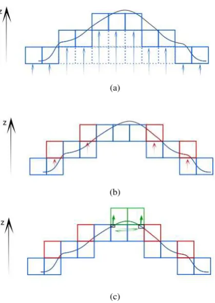
An Octree is used to create the voxel structure. Furthermore, a spatial ID is used to define neighbouring voxels and to search in an ordered list for a voxel of given coordinates. The main at-tribute of ground voxels is, that they are the lowest ones in a local neighbourhood. Therefore, the main idea for a fast voxel based ground detection is to search for the voxel to each x-y- coordinate with the lowest z value. By the use of the octree, this means that within an iteration over all x and y coordinates the ground voxel is found as the first existing voxel inside the iteration from z = 0 to z =2l. A voxel can be seen as a bloated point or as a point group. Therefore, marking only the lowest voxels is like creat-ing samplcreat-ing points in a continuous ground function. Figure 2a illustrates this interpretation as a sampling function.
All voxels have the same size and include different sized areas depending on the voxel sampling. By checking only the low-est voxels, the continuous ground function is transformed to a step function in the voxel space. This could lead to holes in the ground layer (Figure 2a). To avoid these holes, additional voxels are added to the ground if they fulfil the following three condi-tions:
Figure 1. Schematic workflow of the ground detection. Recangles show processing steps and ellipses the output of the
processing step. The gradint calculation is divided into its sub processing steps which are shown in the blue box.
two neighbouring ground voxels with same height do not touch each over (their distance is smaller than a threshold), the next voxels along z are added, as well (see Figure 2c).
The proposed approach can be regarded as a voxel based region growing where step one (Figure 2a) detects seed voxels. After-wards, the region growing is performed between these seeds by looking at the z coordinates of the voxel and determining voxels to be added to the ground segment (Figures 2b and 2c). Roofs and trees create scan shadows inside the ground layer which enables the algorithm to select roof or tree voxels as seeds. Therefore, the ground is over segmented by including roof and tree voxels.
Voxels containing tree points can be selected from this over seg-mented ground by checking the pulse type of all points (pi) in each voxel. Through the number of returns and the return num-ber, it is possible to determine pulse classes, including first, last
(a)
(b)
(c)
Figure 2. The three steps of the ground detection. (a) first step: The lowest existing voxels to each x-y-coordinate (blue ones) are marked as ground voxels. This can be interpreted as creating
sampling points of a continuous ground function (black graph). The blue arrows show the search direction along the z axis and dotted voxels are non existing voxels. (b) second step: adding
voxels where at least one neighbour is marked as ground and have higher or equal z-values. (c) third step: Look if there are sub bounding boxes (black) of the ground voxels which don’t touch each other (green arrows). In this case, the next voxles
along z are added to the ground (marked in green).
and middle pulses (Rutzinger et al., 2008). This is adopted to the point set inside a single voxel. The probability of a voxel to be a voxel consisting of last pulses (to be a ground voxel) is calculated by:
problast=
P i
rnpi P
i
norpi
(1)
where problast= probability of last pulse
withproplast∈[0,1] norpi = number of returns of
the beam to point i
rnpi = return number of point i
Last pulses are the ones, where the return number is equal to the number of returns (Rutzinger et al., 2008). Therefore, this proba-bilty gets a value of 1.0 for a voxel including only last pulses. The probability is smaller than 1.0 if there are other pulse classes in-side the voxel. This behaviour is used to define a threshold which determines voxels including mostly last pulses. Voxels which do not include mostly last pulses are marked as non-ground voxels.
assump-tion that roofs ”fly” over the ground of their local area. The attribute ”fly” symbolizes that there are non existing voxels be-tween the roof and the ground. To search for these roof voxels, a gradient is calculated based on the discrete sampling of the vox-els. This gradient is defined by the biggest difference in height from the current voxel to the closets neighbouring voxels. The closest neighbouring voxels are searched in the list of ground voxels to given x- y-coordinates. A horizontal threshold is used to ignore neighbours inside this list, which are to far away from the current voxel.
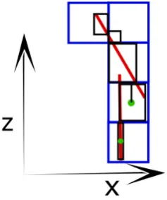
If the ground is flat in the current neighbourhood, the gradient is close to zero, because there is no difference in the height coor-dinates. In case that the current voxel is a roof voxel, the local gradient detects a significant difference of the z-coordinates (Fig-ure 4). The gradient calculation is based on the center points of the sub bounding boxes of neighbouring voxels. These sub bounding boxes are further used to detect facades, which need to be ignored for the gradient calculation. Facades of buildings are detected by looking at the center points of the neighbouring voxels’ sub bounding boxes. If the x-y-coordinates of a center point of a vertical neighbour is inside the horizontal footprint of the current sub bounding box, this neighbour is marked as facade and therefore not considered in the gradient calculation. This fa-cade detection is shown in Figure 3. Figure 4 shows this gradient filter in profile on an example of a roof.
Figure 3. Handling of facade elemets, green line: ground, red line: building, green point: center of the sub bounding box. In case of a neighbour in the vertical direction which includes a facade, the sub bounding box’s center is horizontal inside the current sub bounding box. Such facade including neighbours are
excluded of the list of neighbours.
3.2 Segmentation
The result of the ground detection are two segments: the ground segment and the non-ground segment. The next step is to clus-ter the non-ground segment into smaller parts. The result of this segmentation should be suitable for a further classification task. Therefore, voxels belonging to one segment should have same attributes. For such segmentation, a region growing approach depending on intensity differences as proposed by Aijazi et al. (2013).
Additionally the pulse class of the voxel is used. Withn= number of points, probsingle = probability of single pulse, probfirst =
probability of first pulse andproblast= probability of last pulse,
Figure 4. Profile of the gradient calculation, green line: ground, red line: building. Blue boxes shows the voxel from the octree
and black boxes the sub bounding boxes. The horizontal distance defines usable neighbours and the vertical distance
defines the gradient value.
these pulse classes can be calculated with:
probsingle=Pn
These probabilities are within the range of [0,1]. If the voxel mostly consist of points with the searched pulse class, the proba-bility is close to 1. A segmentation based on the pulse class can be created by putting neighbouring voxels together which have the same pulse class. A single voxel is matched to the pulse class where the probability is above a threshold. The same threshold is used for all probabilities and if all of these probabilities are below this threshold, the voxel consist of middle pulses.
4. DATA
The proposed method is tested on a dataset of the Mangfall area in Bavria, Germany (Figure 5). This area was scanned with a VQ 820G scanner and reaches from the Tegernsee to the highway A8. Approximately 200 Mio points were scanned within three flight strips of approximately 500 m width and 17 km length.
A rotating multi facet mirror is used as the scan mechanism which ensures an incidence angle of 20◦with respect to the flight direc-tion and an accuracy of the incidence angle up to 1◦. The beam divergence is approximately 1 mrad which creates a 50 cm foot-print by a flight height of 500 m (Steinbacher et al., 2012).
Figure 5. The scanned region (Photos from Google maps). In the Background: whole Germany and parts of Europe, in the zoomed part (red rectangle): the scanned Mangfall area (marked
in green) from the Tegernsee in the south to the highway in the north.
(a)
(b)
Figure 6. Region of the Tegernsee. (a): Google Maps Screenshot, (b): Scanned data with the points intensity as grey
value
Beside the intensity (Figure 6) other recognised point attributes are the return number of a single pulse, the number of returns
in the returning signal, the GPS time of the returning signal, the scan angle rank of the laser beam and two flags which indicates the flight strip edges and the scan direction.
5. RESULTS
First algorithmic tests are performed on the Tegernsee part of the proposed data (section 4). This part is shown in Figure 6 and consists of more than 4 mio points. The area has a length of 1.4 km and a width of 400 m. A ground truth (GT) was manually labelled and used for the evaluation. Figure 7 shows the raw data and the ground points inside the ground truth.
(a) (b)
Figure 7. Manually labelled Ground Truth. (a): complete point cloud, (b): ground layer.
For the evaluation of the runtime, different voxel sizes are used. Varying voxel sizes result in different maximum levels of the used octree (Table 1). To reduce the processing time, the whole data set is divided into six smaller parts of equal horizontal dimensions of 500 m by 400 m. These parts are processed in parallel. The resulting accuracies are shown in Figure 8.
The runtime evaluation uses the following parameters:
· Height threshold which determines the voxels to delete in
the gradient chain (Tz): 6 m
· Horizontal threshold, which determines the neighbours to use(Th):0.5·vdiag, wherevdiagis the length of the voxel’s horizontal diagonal.This further addressed as the factor in front ofvdiag.
· Number of iterations for the gradient chain: 30 m /vdiag.
This choice results in a length of 40 m for the gradient chain.
maximum maximum octree level total processing
Voxel size (single thread) time
vx = 20 m
Table 1. Computation time, evaluated on an Intel Core i7-6820HQ CPU
Figure 8. Sensitivity, dependent on the runtime. Different Voxel sizes are symbolized by different run times.
Figure 11 shows that a maximum voxel size of 10 m x 10 m x 1 m creates the best sensitivities. If the voxel size is selected as a smaller or larger one, the sensitivity becomes lower. This has different reasons: In the case of larger voxels, the point cloud is more generalized. Therefore, the selection of a voxel to be a non-ground voxel will excise more points of the ground layer. This is shown by a strong fall of the function for the detected ground points. In contrast to larger voxels, smaller voxels pre-serve more details in the point cloud generalisation. In the case of smaller voxels, the scan shadows of buildings inside the ground layer are preserved as well and more seed voxels are selected on roofs. Due to more details, it is possible that the gradient gets with small steps to the ground and therefore preserve these wrongly detected ground voxels. In other words, the wrongly tected ground is not detected non-ground, which explains the de-crease of the non-ground sensitivity. Especially the z-dimension becomes very small with higher octree levels, because the initial bounding box has a smaller z-dimension than x- or y- dimension. Voxels with very small z-dimensions create a sparse height sam-pling of the ground layer and therefore create unoccupied voxels between two ground voxels. The region growing is aborted at these unoccupied voxels and the sampling of the ground layer is less complete, too. Since figure 11 shows the sensitivities of both classes, the accuracies can be estimated as well. The ab-solute number of ground points in the GT-data is: 2131236 and the absolute number of non-ground points: 2330592. By using this values to calculate the accuracies of the two classes, it turns out, that the accuracy of the one class is close to the sensitivity of the other class. Therefore, the following evaluation of the filter method uses only the sensitivity values.
Figure 11 shows a comparison of the influence of two major pa-rametersTz andThof the used filter. The used maximum voxel sizes are 10 m x 10 m x 1 m and 3 m x 3 m x 1 m. The func-tion graphs of these two maximum voxel sizes look similar which means, that the influence ofTz andThbehaves the same. The stronger generalisation by larger voxels and the resulting elimi-nation of more points of the ground layer is shown by the off-set and bigger differences between the two sensitivity graphs. In general it can be said, that a lowerTzwith higherThresults in a higher sensitivity of the non-ground segment. This configuration results in a stronger filter and therefore in more detected outliers. The lower sensitivity of the ground layer can be explained by a stronger filter, too. Since steep slopes and roofs are very similar in the scanner data (both have big height differences in a small area), a stronger filter will delete the points of steep slopes as well as roof points. Therefore, the sensitivities are correlated in a negative manner. If the sensitivity of the non-ground layer gets bigger, the sensitivity of the ground layer gets lower. The influ-ence ofThdepends on the value ofTz. IfTz is selected to be lower,Thchanges the sensitivities with a stronger influence.
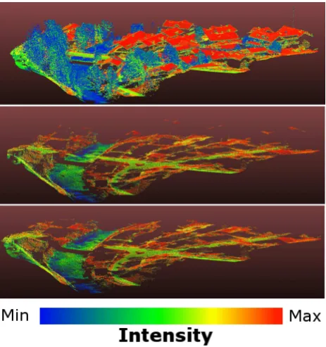
A visual result of the proposed method is shown in Figure 9. This figure shows the area of the northern bridge across the river (see Figure 7) with a view direction from north to south. The used maximum voxel dimension is 10 m x 10 m x 1 m and the used filter parameters are:Tz= 6 m,Th= 0.5.
Figure 9. Results of the ground detection. Top: raw data, middle: result of our approach, bottom: ground truth
This area was selected, because it shows some remaining roof points in the ground layer. The area includes steep slopes below vegetation as well as water and river bed points. Both configura-tions can be handled with the proposed method as it can be seen in the figure.
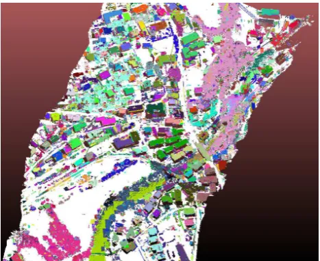
Figure 10. Result of the segmentation of the non-ground segment. The maximum Voxel dimension is x,y<20m, z<2m.
The segments in the point clouds are colour coded: white: ground, others: randomly different color.
6. SUMMARY
This paper introduces a geometric segmentation approach for air-borne multi-response LIDAR data. Since such airair-borne data can become very large (a large amount of points is scanned), a voxel structure is used to generalize the data and therefore reduce pro-cessing time. This voxel structure is used for a ground segmenta-tion.
The proposed ground detection is able to detect the ground of a hilly terrain as well as the ground below vegetation and water surfaces. By using the voxel generalization, the ground detection is almost independent of the number of points inside the point cloud. The experimented results revealed that the performance and processing time depend on the used voxel size.
Some over and under segmentations of the ground still exist. Un-der segmentations are characterized by small non-ground areas surrounded by ground points. Over segmentations are charac-terized by ground areas surrounded by roof points. This phe-nomenon will be used to detect and correct the over and under segmentations in the future by checking the class labels of the local neighbourhood.
The segmentation results of non-ground areas (Figure 10) are cre-ated by a segmentation dependent on the voxel pulse classes: sin-gle, first, middle or last pulse. This segmentation shows a cut of vegetation areas into tree crown top points and other tree points. A combination of pulse class and intensity difference should be considered for the segmentation in future work. Furthermore, the segmentation of non-ground areas will be used for a classification task, which matches each segment to the class labels: building, vegetation and water.
ACKNOWLEDGEMENTS
This research is funded by Bayerische Forschungsstriftung, project ”Schritthaltende 3D-Rekonstruktion und -Analyse (AZ-1184-15)”, sub project ” ¨Anderungsdetektion in Punktwolken”. The dataset is provided by our project partner SteinbacherCon-sult.
REFERENCES
Aijazi, A. K., Checchin, P. and Trassoudaine, L., 2013. Segmen-tation based classification of 3D urban point clouds: A super-voxel based approach with evaluation. Remote Sensing 5(4), pp. 1624–1650.
European Union, 2000. Directive 2000/60/EC of the European Parliament and of the Council of 23 October 2000 establishing a framework for Community action in the field of water policy. http://eur-lex.europa.eu/legal-content/DE/TXT/?uri=CELEX(29 Nov. 2016).
European Union, 2007. Directive 2007/60/EC of the Euro-pean Parliament and of the Council of 23 October 2007 on the assessment and management of flood risks. http://eur-lex.europa.eu/legal-content/DE/TXT/?uri=CELEX(29 Nov. 2016).
Hebel, M. and Stilla, U., 2009. Automatische Koregistrierung von ALS-Daten aus mehreren Schr¨agansichten st¨adtischer Quartiere. Photogrammetrie Fernerkundung Geoinformation3, pp. 261–275.
Hebel, M. and Stilla, U., 2012. Simultaneous calibration of ALS systems and alignment of multiview LiDAR scans of urban
ar-eas.IEEE Transactions on Geoscience and Remote Sensing5(6),
pp. 2364–2379.
Mandlburger, G., Hauer, C., Wieser, M. and Pfeifer, N., 2015. Topo-bathymetric LiDAR for monitoring river morphodynamics and instream habitats - a case study at the pielach river. Remote
Sensing7(5), pp. 6160–6195.
Niemeyer, J., Rottensteiner, F. and Soergel, U., 2014. Contextual classification of lidar data and building object detection in urban areas.ISPRS journal of photogrammetry and remote sensing87, pp. 152–165.
Reitberger, J., Schn¨orr, J., Krzystek, P. and Stilla, U., 2009. 3D segmentation of single trees exploiting full waveform lidar data.
ISPRS Journal of Photogrammetry and Remote Sensing64(6),
pp. 561–574.
Rutzinger, M., H¨ofle, B., Hollaus, B. and Pfeifer, N., 2008. Object-based point cloud analysis of full-waveform airborne laser scanning data for urban vegetation classification. Sensors8(8), pp. 4505–4528.
Shapovalov, R., Velizhev, A. and Barinova, O., 2010. Non-associative markov networks for 3D point cloud classification.
The International Archives of the Photogrammetry, Remote
Sens-ing and Spatial Information Sciences.
Steinbacher, F., Pfennigbauer, M., Aufleger, M. and Ullrich, A., 2012. High resolution airborne shallow water mapping. In:
International Archives of the Photogrammetry, Remote Sensing and Spatial Information Sciences, Proceedings of the XXII ISPRS
Congress, Vol. 39, p. B1.
Xu, Y., Tuttas, S. and Stilla, U., 2016. Segmentation of 3d out-door scenes using hierarchical clustering structure and perceptual grouping laws. In: 2016 9th IAPR Workshop on Pattern
Recog-niton in Remote Sensing (PRRS), pp. 1–6.
Xu, Y., Tuttas, S., Hoegner, L. and Stilla, U., 2017. Geometric primitive extraction from point clouds of construction sites us-ing vgs. IEEE Geoscience and Remote Sensing Letters14(3), pp. 424–428.
Zhang, Z., Zhang, L., Tong, X., Mathiopoulos, P. T., Guo, B., Huang, X., Wang, Z. and Wang, Y., 2016. A multilevel point-cluster-based discriminative feature for ALS point cloud classi-fication. IEEE Transactions on Geoscience and Remote Sensing
maximum Voxel dimension: 3 m x 3 m x 1 m maximum Voxel dimension: 10 m x 10 m x 1 m