CLASSIFICATION AND MODELLING OF URBAN MICRO-CLIMATES USING
MULTISENSORAL AND MULTITEMPORAL REMOTE SENSING DATA
B. Bechtel a, *, T. Langkamp a, J. Böhner a, C. Daneke a, J. Oßenbrügge a, S. Schempp a
a
KlimaCampus, University of Hamburg, Bundesstraße 55, 20146 Hamburg, Germany –
benjamin.bechtel@uni-hamburg.de
Commission VIII/8: Land
KEY WORDS: Urban, Climate, Human Settlement, Classification, Thermal, DEM/DTM, Landsat
ABSTRACT:
Remote sensing has widely been used in urban climatology since it has the advantage of a simultaneous synoptic view of the full urban surface. Methods include the analysis of surface temperature patterns, spatial (biophysical) indicators for urban heat island modelling, and flux measurements. Another approach is the automated classification of urban morphologies or structural types. In this study it was tested, whether Local Climate Zones (a new typology of thermally 'rather' homogenous urban morphologies) can be automatically classified from multisensor and multitemporal earth observation data. Therefore, a large number of parameters were derived from different datasets, including multitemporal Landsat data and morphological profiles as well as windowed multiband signatures from an airborne IFSAR-DHM.
The results for Hamburg, Germany, show that different datasets have high potential for the differentiation of urban morphologies. Multitemporal thermal data performed very well with up to 96.3 % overall classification accuracy with a neuronal network classifier. The multispectral data reached 95.1 % and the morphological profiles 83.2 %.The multisensor feature sets reached up to 97.4 % with 100 selected features, but also small multisensoral feature sets reached good results. This shows that microclimatic meaningful urban structures can be classified from different remote sensing datasets.
Further, the potential of the parameters for spatiotemporal modelling of the mean urban heat island was tested. Therefore, a comprehensive mobile measurement campaign with GPS loggers and temperature sensors on public buses was conducted in order to gain in situ data in high spatial and temporal resolution.
* Corresponding author.
1. INTRODUCTION
Urban climatology is an important application for remote sensing of urban areas. The growing interest in urban climatic phenomena like the urban heat island (UHI) is motivated by increasing vulnerability to health risks due to rapid urbanization in developing countries and climate change.
The urban heat island indicates increased air temperatures in the urban atmosphere compared to a preurban state (Lowry, 1977) or (more often) to a rural reference station of identical regional and topo-climate. It is the most prominent effect of urban climate (Oke, 1982; Arnfield, 2003; Yow, 2007) and has been studied more intensely than any other effect. The UHI varies both diurnally and seasonally and depends on the prevailing synoptic conditions. It is particularly pronounced at low wind speeds and high air pressure (Oke, 1973) and has been documented for many towns and cities of different sizes and on different continents (Oke, 1982). Further, it depends on the size of the city (Oke, 1973). Within a city the UHI greatly varies depending on the urban structure and vegetation and is therefore also referred to as urban heat archipelago.
Remotely sensed data can contribute to descriptive urban climatic studies and a better understanding of the underlying climatic processes. The assessment of surface atmosphere exchanges (Rigo and Parlow, 2007) was fostered by recent advances in earth observation technologies. Further, remote sensing has widely been applied to characterise the urban surface and to determine parameters for model and experimental studies. Thus, fundamental physical attributes of
measurement sites and key parameters for urban climate models can be derived from remotely sensed data (Grimmond, 2006). This includes parameters of the urban energy balance like albedo and emissivity (Frey et al., 2007; Frey and Parlow, 2009), the urban canyon geometry, and aerodynamic characteristics like roughness parameters (Bechtel et al., 2011). Further, automated classification of urban structures in respect to their microclimatic properties can contribute to urban climate studies. A typology of such thermally defined urban structures was recently introduced with the Local Climate Zones (LCZ) scheme (Stewart and Oke, 2009).
Great attention has been devoted to the application of thermal infrared data for UHI assessment (Roth et al., 1989; Eliasson, 1992; Gallo and Owen, 1999; Voogt and Oke, 2003; Nichol et al., 2009; Wong et al., 2009; Fabrizi et al., 2011). Thermal imagery offers the chance to directly measure the surface temperature which is crucial for the urban energy balance and modulates the air temperature of the lowest atmospheric layer. Therefore, the spatial structure of the surface temperature patterns is not only directly related to surface characteristics but also used to study the energy balance and the relation between atmospheric heat island and surface temperature heat island (Voogt and Oke, 2003). However, there are various problems involved in linking thermal imagery to air temperatures which mostly remain unsolved (Roth et al., 1989; Voogt and Oke, 1997; Voogt and Oke, 2003).
Beside recent advances in the development of surface parameters for assessing the urban thermal response, “new methods for estimation of UHI parameters from multi-temporal
and multi-location TIR imagery are still needed” (Weng, 2009, p. 340) and the measurement of the urban heat island remains difficult. In (Bechtel and Schmidt, 2011) a large set of predictors was compared with a long-term UHI dataset derived from floristic proxy data and classical parameters like surface temperature and NDVI were found useful.
In this study different (multitemporal) parameter sets were tested for their potential to classify thermal LCZ (see Bechtel and Daneke, 2012 for more detail) and derive empirical models of the mean UHI from a mobile measurement campaign.
2. DATA
The city of Hamburg in Northern Germany was chosen as site for the case study. The full domain covers 1132 km².
2.1 Multisensor and multitemporal features
Due to its high availability a strong emphasis was laid on multitemporal Landsat TM and ETM+ data in this study. This reflects on the different phenological conditions throughout the year and the thermal response to different insulation conditions which both reveal additional information. A disadvantage is possible land cover change within the acquisition period which may lead to classification errors. However, this is expected to be acceptable since a high degree of persistence can be assumed for the study area at the temporal scale of decades. The multitemporal data were complemented with geometrical and texture data from NEXTMap® Interferometric Synthetic Aperture Radar (IFSAR). Overall seven feature sets were compiled (see Table 1) and projected to a common 100 m grid with SAGA (www.saga-gis.org). The parameters are also named features (for classification) or predictors (for empirical modelling) in the following.
The multitemporal multispectral (MS) parameters were derived from 33 visually cloud-free scenes acquired between 1987 and 2010 (see Bechtel, 2011 for a detailed description of the preprocessing). All spectral bands (1–5 & 7, ranging from blue ~485 nm to medium infrared 2.2 µm) were included in the feature set. For each scene the Normalized Differenced Vegetation Index (NDVI) was computed from the bands 3 and 4 as an additional band ratio. Atmospheric influence was neglected, since the parameters were only used in trained classifiers and models and no information about subscene atmospheric conditions was available.
The multitemporal thermal infrared (TIR) data from TM and ETM+ (Band 6, 10.4–12.5 µm) was processed accordingly. Digital numbers were used directly as features (without atmospheric correction and calibration to radiance) for the same reason. Further, surface temperatures were calculated for 22 scenes with National Centers for Environmental Prediction (NCEP) atmospheric profiles available (Barsi et al., 2005, Chander et al., 2009) in order to fit a simple model of the annual cycle of temperature at acquisition time. The annual cycle parameters (ACP) Yearly Amplitude of Surface Temperature (YAST) and Mean Annual Surface Temperature (MAST) contain information about the material specific thermal surface properties (Bechtel, 2011; Bechtel, 2012).
The geometric parameters were derived from a normalised digital height model generated from NEXTMap® Digital Surface and Terrain Model on a 3 m grid. Besides simple statics of the obstacle heights, further parameters were extracted by Fourier techniques and morphologic filtering, in order to derive spatial spectra and texture information and thus include spatial information in the pixel-based classification approach (see Bechtel and Daneke, 2012 for more details).
param category description number
ms mt ms multispectral (TM/ETM+ ) 198
ndvi mt ms ndvi 33
tir mt tir thermal (TM/ETM+ ) 33
acp mt tir annual cycle parameters 2 shs geom simple height statistics 6 morph geom morphological profiles (texture) 22 fft geom bandpass & directional filters 190
overall 484
Table 1. Feature sets and number of features per set.
2.2 Training data – Local Climate Zones
The LCZ scheme is a local-scale landscape classification system based on the thermal properties of urban structural types (Stewart and Oke, 2009) and has high potential to become a standard in urban climatology. The four basic landscapes series (city, agricultural, natural and mixed) are each subdivided according to their microscale (10s–100s of meters) surface properties (more specifically: sky view factor, fraction of impervious materials, Davenport roughness class, surface thermal admittance and mean annual anthropogenic heat flux) which affect the canopy-layer thermal climate. Since the typology has a certain cultural bias towards Northern American morphologies a compatible but slightly adopted scheme was used for this study. For all classes representative reference areas were digitized on a 100 m grid using map and high resolution optical remote sensing data.
The urban series was subdivided into eleven categories. Urban Core (urbcore) is representing the historic inner city with massive buildings of uniform height with single spires like bell towers. The compact morphologies were split into the classes Urban Dense (urbdens) with perimeter block buildings of uniform height with courtyards in the center and Terraced Housing (terrace) with a regular pattern aligned in rows. Blocks
refer to clustered high-rise buildings in a uniform geometric layout while Modern Core (modcore) comprises high rise commercial buildings. Regular Housing (reghous) consists of single family houses with a high proportion of greening between the spaces and is typical for suburbs. The industrial areas are divided into Industry (industr) with industrial or commercial activities in low-rise buildings and Port (port)
which also contains container-arrays and storage facilities beside similar structures. Rail tracks (rail), park and gardens
complement the urban series. From the natural and agricultural series field, forest and water bodies were found relevant for the area of interest.
2.3 UHI data
The UHI data was collected during a mobile measurement campaign with public transportation buses in Hamburg during the vegetation period from the 23rd of May until the 29th of October 2011. Cooperation with the Hochbahn Hamburg allowed for the collection of spatially dense air temperature data in the inner city of Hamburg. Therefore, 15 buses were equipped with temperature (and humidity) sensors of Driesen & Kern. These sensors show a very fast responsiveness to temperature changes which is necessary due to the fast movement of the buses (up to 90 km/h). The DK311 loggers were combined with CO-325 temperature sensors, RFT325 humidity sensors and a radiation protection shields. The position was recorded with Qstarz BT-Q1000XT GPS-loggers powered by the mobile power pack VT-PP-320 by Variotek. International Archives of the Photogrammetry, Remote Sensing and Spatial Information Sciences, Volume XXXIX-B8, 2012
They were contained in a waterproof OtterBox 3000 case and mounted magnetically on the front roof, where the temperature influence of the bus itself was smallest (tested with surface-temperature-sensors at three positions of the roof). This construction allowed for continuous measuring for five to six days (5 seconds intervals for temperature and 20 meters intervals for position and velocity).
Since the air temperature measurements can be contaminated by the roof temperature of the bus at low travelling speeds, data collected at velocities lower than 12 km/h were discarded in the post-processing. Then, the temperature data were linearly interpolated to a frequency of one second and matched with the according time stamps of the GPS data. To reduce the massive dataset, the single measurements were then averaged to one minute intervals and aggregated to an network of virtual stations with approximately 100m spacing (derived from the centers of all measurements within a regular 100 m-grid).
Subsequently, the data were transferred to a PostgreSQL / PostGIS database and validated with data of 25 stationary measurement sites from various sources. The comparison of the mobile measurements with near stationary measurements (distance < 130 m, +/- 2.5 minutes, n=108) revealed a satisfactory quality of the collected data with a mean difference between stationary and mobile measurements of -0.15 K and a mean absolute error of 0.51 K. The UHI was then calculated as the difference to stationary measurements from the Hamburg Weather Mast operated by the Meteorological Institute of the University of Hamburg. Although this data is likely to contain some urban effects, the offset to the ‘real’ UHI could be neglected for this study.
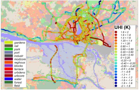
To guarantee a minimum of comparability, ‘stations’ with less than 30 individual measurements were excluded from the subsequent analysis. For the remaining 1260 virtual stations the mean UHI was calculated from all individual measurements. The UHI data are shown in Figure 1.
Figure 1. Mean UHI data from the mobile measurement campaign with public transportation buses. Circle size indicates
the number of measurements.
3. METHODS
3.1 Feature selection
For feature selection the Minimum Redundancy Maximal Relevance approach (MRMR) approach was chosen, which was originally developed in bioinformatics for genome classification (Peng et al., 2005). The algorithm selects features that have both high relevance for classification of the target classes and low redundancy with the prior selected features; the distance between two features is defined by their mutual information. For this study the Mutual Information Quotient (MIQ) criterion was used.
p(x, y) = joint probabilistic distribution p(x), p(y) = marginal probabilities
3.2 Classifiers
Six supervised classifiers (implemented in the Waikato environment for knowledge analysis data mining package; Bouckaert et al., 2009) were used in this study.
The Naive Bayes (NB) classifier assumes conditional
independency, which reduces the posterior probability of class membership to the product of the estimate of the features’ marginal probabilities. Despite its simplicity it often delivers good results. The Support Vector Machine (SVM) classifier transfers the problem to pairwise classification in a higher dimensional space (Burges, 1998). The Multilayer Perceptron
classifier is a feedforward artificial neural network (NN) composed by nodes (neurons) in connected layers. It is trained by a backpropagation algorithm. The Random Forest (RF) classifier utilises a number of tree-structured classifiers as committee to decide with majority and shows excellent classification performance and computing efficiency. The single trees are each generated from a random subset and therefore an ‘out of bag’ error can be estimated without any bias. The number of trees grown and the number of features used for each tree were varied and three configurations were tested. While RF1 worked with 10 trees, RF2 used 30 trees and 20 features, and RF3 50 trees and 30 features (see Bechtel and Daneke, 2012 for more detailed information).
3.3 Empirical models
For the evaluation of the UHI data two different empirical models were used. For the Linear Regression (LR) model attributes were selected by the M5 method and collinear attributes were eliminated. The Multilayer Perceptron is again a neuronal networks trained by a backpropagation algorithm, but this time predicts a numerical value instead of class membership probabilities.
4. RESULTS
4.1 Classification of LCZ
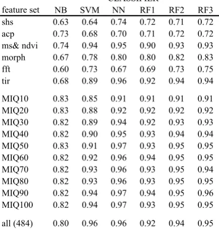
Table 2 shows the classification results for classifiers and feature sets. All numbers refer to the overall accuracy evaluated International Archives of the Photogrammetry, Remote Sensing and Spatial Information Sciences, Volume XXXIX-B8, 2012
with a testing sample of about 25 % of the digitized input data for each class. The training pixels where neither used in the MRMR feature selection nor in the classifier training. The first lines refer to the feature sets in Table 2, the second part to feature sets of different sizes selected with the MRMR algorithm and the MIQ criterion.
The results are quite convincing. The thermal data performed best of all feature sets from one sensor (with up to 96.3 % overall classification accuracy with the Multilayer Perceptron classifier). This is quite consequent, considering the thermal definition of the LCZ. The multispectral data also reached very good results (95.1% with Multilayer Perceptron), while the simple heights (74.0 % with Multilayer Perceptron), the bandpass & directional filters (74.8 % with Random Forest) and the morphological profiles (83.2 % with Random Forest) performed less well.
The multisensor feature sets reached up to 97.4 % (with Multilayer Perceptron and 100 features), but also small multisensoral feature sets reached good results (up to 92.5 % with 20, 93.7 % with 30, 94.9 % with 40 and 96.7 % with 50 features). These results are comparable to other studies (c.f. Bechtel and Daneke, 2012).
Regarding the different classifiers, Multilayer Perceptron showed the best results, but considering the much higher computing costs Random Forest seems a suitable and fast alternative (and can be assumed to be more robust and not overfitting). The Support Vector Machine classifiers performs worse than NN and RF for smaller feature sets but takes most benefit of further features (for all other classifiers the accuracy is higher for 100 selected features than for the full feature set). Naïve Bayes performs less well than the highend classifiers and takes less advantage of further features (since the conditional independence assumption is violated with increasing redundancy in the feature set).
Figure 2 shows the classification result for the full domain with the Multilayer Perceptron classifier and 100 selected multisensoral features. The visual evaluation reveals a very high accordance with the existing urban and natural structures.
feature set NB SVM NN RF1 RF2 RF3
shs 0.63 0.64 0.74 0.72 0.71 0.72
acp 0.73 0.68 0.70 0.71 0.72 0.72
ms& ndvi 0.74 0.94 0.95 0.90 0.93 0.93 morph 0.67 0.78 0.80 0.80 0.82 0.83
fft 0.60 0.73 0.67 0.69 0.73 0.75
tir 0.68 0.89 0.96 0.92 0.94 0.94
MIQ10 0.83 0.85 0.91 0.91 0.91 0.91 MIQ20 0.83 0.88 0.92 0.92 0.92 0.92 MIQ30 0.82 0.89 0.94 0.92 0.93 0.93 MIQ40 0.82 0.90 0.95 0.93 0.94 0.94 MIQ50 0.83 0.91 0.97 0.93 0.95 0.95 MIQ60 0.82 0.92 0.96 0.94 0.95 0.95 MIQ70 0.82 0.93 0.96 0.93 0.95 0.94 MIQ80 0.82 0.93 0.96 0.93 0.95 0.95 MIQ90 0.82 0.94 0.97 0.94 0.95 0.96 MIQ100 0.82 0.94 0.97 0.93 0.95 0.95
all (484) 0.80 0.96 0.96 0.92 0.94 0.95 CLASSIFIER
Table 2. Classification results for different feature sets including multisensoral feature sets selected with the MRMR
MIQ criterion.
Figure 2. LCZ classification with NN classifier and 100 multisensoral features selected by MRMR (MIQ). Mixed
classes overlay was digitized from map data.
4.2 Empirical UHI model
Further, the potential of the multitemporal und multisensoral parameter sets for spatiotemporal modelling of the mean UHI was tested with Linear Regression and Multilayer Perceptron models. The results are shown in Table 3. The models were again evaluated with a randomly chosen testing sample of about 25 % of all stations, which was not used in prior model calibration.
As for the classification the multitemporal thermal (correlation R of 0.74/0.81 and mean absolute error of 0.17/0.19 K for Linear Regression and Neuronal Network) and the multitemporal spectral (R 0.75/0.77, MAE: 0.17/0.19 K) data performed better than the simple height statistics (R: 0.27/0.26, MAE: 0.24/0.26 K) and the annual cycle parameters (R: 0.19/0.18, MAE: 0.24/0.24 K). This is, certainly partly a consequence of the different parameter set sizes.
Although an error of only about 0.2 K in the predicted mean UHI seams promising at the first glance, the quality of the empirical models is not yet satisfying in respect to the low spatial variance in the dataset (even for the better models this corresponds to an relative error of about 60 %). This is not surprising regarding the large number of processes contributing to alterations in the urban atmosphere. Those effects are related to the urban structure, vegetation, and surface temperature in different ways and hence only very indirectly to the multispectral and thermal data. However, the multispectral data comprises different insulation and phenological conditions and this information can be utilised during the model calibration. Multisensoral data including thermal, spectral and height features performed better than sets from the same sensor. However, this was not the case for preselected features with high individual relevance (R > 0.25), which might indicate a certain redundancy. Further, the testing sample might not be completely independent, since close stations are likely to be correlated.
Parameter set
N R MAE RMSE R MAE RMSE
shs 6 0.27 0.24 0.32 0.26 0.26 0.33
acp 2 0.19 0.24 0.32 0.18 0.24 0.32
tir 33 0.74 0.17 0.22 0.81 0.19 0.23 ndvi 33 0.66 0.19 0.25 0.70 0.21 0.28 ms 198 0.75 0.17 0.22 0.77 0.18 0.23 R>.25 71 0.71 0.18 0.23 0.73 0.18 0.25 all 272 0.79 0.16 0.21 0.82 0.15 0.2
LR NN
Table 3. Results of the spatial empirical models (Linear Regression and Neuronal Network) of the mean UHI with different parameter/predictor sets. Correlation coefficient R,
mean absolute error and root mean square error.
Nevertheless, it can be stated, that multisensoral and multitemporal datasets have some potential for spatiotemporal modelling of the mean UHI. This underlines the results of Bechtel and Schmidt, who found strong correlations between Landsat data and a long-term mean UHI dataset derived from floristic proxy data (Bechtel and Schmidt, 2011).
The performance of Linear Regression and Neuronal Network models was rather similar, which might be due to the chosen standard options for the neuronal network classifier (with only one hidden layer). First tests with more sophisticated networks showed better results (for instance R: 0.83, MAE: 0.14 K for tir with a 20|10|10 node network).
5. CONCLUSIONS
The presented results from Hamburg indicate that multisensoral and multitemporal data has potential for both, the classification of Local Climate Zones and the empirical modelling of the spatial distribution of the UHI.
The classification results show that the data (especially multitemporal thermal and multitemporal spectral data) are functional for the purpose and that micro-climatic meaningful urban structures can be classified from different remote sensing datasets. Further, it provides some evidence for the relevance of the Local Climate Zone system from a remote sensing point of view.
The empirical modelling results also underpin the urban climatologic relevance of the multitemporal tir und ms data. Although a certain correlation is obvious, since vegetation and surface energy balance play important roles in the distinction of urban climates, these good results with freely available Landsat data offer the prospect of a wide application. However, further investigations are needed and the large number and complexity of the involved processes limits the potential of empirical models. The incorporation of data from other sensors also slightly improved the empirical modelling results.
6. REFERENCES
Arnfield, A. J., 2003. Two decades of urban climate research: a review of turbulence, exchanges of energy and water, and the urban heat island. International Journal of Climatology, 23(1), pp. 1–26.
Barsi, J. A., Schott, J. R., Palluconi, F. D., and Hook, S. J., 2005. Validation of a Web-Based atmospheric correction tool for single thermal band instruments. Earth Observing Systems
X, Proc. SPIE, 58820E, pp. 1–7.
Bechtel, B., 2011. Multitemporal Landsat data for urban heat island assessment and classification of local climate zones.
Urban Remote Sensing Event, JURSE, 2011 Joint, pp. 129–132.
doi:10.1109/JURSE.2011.5764736.
Bechtel, B., 2012. Robustness of Annual Cycle Parameters to characterize the Urban Thermal Landscapes. IEEE Geoscience
and Remote Sensing Letters, doi 10.1109/LGRS.2012.2185034.
Bechtel, B. and Daneke, C., 2012, Classification of local Climate Zones based on multiple Earth Observation Data. IEEE Journal of Selected Topics in Applied Earth Observations and Remote Sensing. doi 10.1109/JSTARS.2012.2189873.
Bechtel, B., Langkamp, T., Ament, F., Bohner, J., Daneke, C., Gunzkofer, R., Leitl, B. et al., 2011. Towards an urban roughness parameterisation using interferometric SAR data taking the Metropolitan Region of Hamburg as an example.
Meteorologische Zeitschrift, 20(1), pp. 29–37.
Bechtel, B., and Schmidt, K., 2011. Floristic mapping data as a proxy for the mean urban heat island. Climate Research, 49, pp. 45-58. doi:10.3354/cr01009
Bouckaert, R. R., Frank, E., Hall, M., Kirkby, R., Reutemann, P., Seewald, A., and Scuse, D., 2009. WEKA manual for version 3-7-0. University of Waikato, Hamilton, New Zealand. Disponible en: http://ufpr. dl. sourceforge.
net/project/weka/documentation/3.7. x/WekaManual-3-7-0. pdf.
Burges, C. J. C., 1998. A tutorial on support vector machines for pattern recognition. Data mining and knowledge discovery, 2(2), pp. 121–167.
Chander, G., Markham, B. L., and Helder, D. L., 2009. Summary of current radiometric calibration coefficients of Landsat MSS, TM, ETM+ and EO-1 ALI Sensors. Remote
Sensing of Environment, 113, pp. 893–903.
Eliasson, I., 1992. Infrared thermography and urban temperature patterns. International Journal of Remote Sensing, 13, pp. 869–879.
Fabrizi, R., De Santis, A., and Gomez, A., 2011. Satellite and ground-based sensors for the Urban Heat Island analysis in the city of Madrid. Urban Remote Sensing Event, JURSE, 2011
Joint. doi:10.1109/JURSE.2011.5764791
Frey, C., and Parlow, E., 2009. Geometry effect on the estimation of band reflectance in an urban area. Theoretical and
Applied Climatology, 96(3), pp. 395–406.
Frey, C., Rigo, G., and Parlow, E., 2007. Urban radiation balance of two coastal cities in a hot and dry environment.
International Journal of Remote Sensing, 28(12), pp. 2695–
2712.
Gallo, K. P., and Owen, T. W., 1999. Satellite-Based Adjustments for the Urban Heat Island Temperature Bias.
Journal of Applied Meteorology, 38(6), pp. 806–813.
Grimmond, C. S. B., 2006. Progress in measuring and observing the urban atmosphere. Theoretical and applied
climatology, 84(1), pp. 3–22.
Lowry, W. P., 1977. Empirical estimation of urban effects on climate: A problem analysis. J. Appl. Meteorol., 16, pp. 129– 135.
Nichol, E. J., Fung, W. Y., Lam, K. S., and Wong, M. S., 2009. Urban heat island diagnosis using ASTER satellite images and „in situ“ air temperature. Atmospheric Research, 94, pp. 276– 284.
Oke, T. R., 1973. City size and the urban heat island.
Atmospheric Environment, 7, pp. 769–779.
Oke, T. R., 1982. The energetic basis of the urban heat island.
Quaterly J. Royal Meterol. Soc., 108, pp. 1–24.
Peng, H., Long, F., and Ding, C., 2005. Feature Selection Based on Mutual Information: Criteria of Dependency, Max-Relevance, and Min-Redundancy. IEEE Transactions on
Pattern Analysis and Machine Intelligence, 27(8), pp. 1226–
1238.
Rigo, G., and Parlow, E., 2007. Modelling the ground heat flux of an urban area using remote sensing data. Theoretical and
Applied Climatology, 90(3-4), pp. 185–199.
doi:10.1007/s00704-006-0279-8
Roth, M., Oke, T. R., and Emery, W. J., 1989. Satellite-derived urban heat islands from three coastal cities and the utilization of such data in urban climatology. International Journal of
Remote Sensing, 10(11), pp. 1699–1720.
Stewart, I.D., and Oke, T. R., 2009. Newly developed “thermal climate zones” for defining and measuring urban heat island magnitude in the canopy layer. Preprints, T.R. Oke Symposium and Eighth Symposium on Urban Environment, January 11–15, Phoenix, AZ.
Voogt, J. A., and Oke, T. R., 1997. Complete Urban Surface Temperatures. J. Appl. Meteorol., 36(9), pp. 1117–1132.
Voogt, J. A., and Oke, T. R., 2003. Thermal remote sensing of urban climates. Remote Sensing of Environment, 86, pp. 370– 384.
Weng, Q., 2009. Thermal infrared remote sensing for urban climate and environmental studies: Methods, applications, and trends. ISPRS Journal of Photogrammetry and Remote Sensing, 64(4), pp. 335–344.
Wong, M. S., Nichol, J., and Kwok, K. H., 2009. The urban heat island in Hong Kong: causative factors and scenario analysis. Urban Remote Sensing Event, 2009 Joint, JURSE. doi: 10.1109/URS.2009.5137468.
Yow, D. M., 2007. Urban heat islands: observations, impacts, and adaptation. Geography Compass, 1(6), pp. 1227–1251.
7. ACKNOWLEDGEMENTS
We are grateful to T. Bluemel and the Hochbahn Hamburg for the cooperation in the bus measurement campaign, to I. Lange and B. Brümmer for the Wettermast data as well as all further providers of station data used for the validation of the bus measurements. For remote sensing data we thank the NASA and Intermap Technologies. Further, we thank H. Peng and colleagues for the MRMR code, the Machine Learning Group at the University of Waikato for WEKA as well as O. Conrad and the SAGA user group for SAGA.