ARCHETYPAL ANALYSIS FOR SPARSE REPRESENTATION-BASED
HYPERSPECTRAL SUB-PIXEL QUANTIFICATION
Lukas Dreesa∗, Ribana Roschera
a
Institute of Geodesy and Geoinformation, Remote Sensing Group, University of Bonn, Germany - (s7ludree, ribana.roscher)@uni-bonn.de
KEY WORDS:Archetypal analysis, sparse representation, sub-pixel quantification
ABSTRACT:
This paper focuses on the quantification of land cover fractions in an urban area of Berlin, Germany, using simulated hyperspectral EnMAP data with a spatial resolution of30m×30m. For this, sparse representation is applied, where each pixel with unknown surface characteristics is expressed by a weighted linear combination of elementary spectra with known land cover class. The elementary spectra are determined from image reference data using simplex volume maximization, which is a fast heuristic technique for archetypal analysis. In the experiments, the estimation of class fractions based on the archetypal spectral library is compared to the estimation obtained by a manually designed spectral library by means of reconstruction error, mean absolute error of the fraction estimates, sum of fractions and the number of used elementary spectra. We will show, that a collection of archetypes can be an adequate and efficient alternative to the spectral library with respect to mentioned criteria.
INTRODUCTION
The estimation of the degree of imperviousness as an indicator of environmental quality is subject of current research towards a time and cost efficient monitoring of urban areas (Weng, 2012). Remote sensing data, such as imaging spectroscopy, builds a valuable basis to comprehensively map urban areas and quan-tify the imperviousness based on the spectral information (e.g., Huang et al. (2014); Roessner et al. (2011)). Especially, hyper-spectral imagery is a well suited source for mapping of such ar-eas, because it offers a high spectral separability of different ma-terials. However, generally, the temporal and spatial resolution is limited in comparison to sensors with lower spectral resolu-tion. These limitations are partially overcome with the launch of missions such as Environmental Mapping and Analysis Program (EnMAP), which increases the availability of hyperspectral data and therefore the temporal resolution (Guanter et al., 2015). Nev-ertheless, due to its spatial resolution, the provided data is mainly characterized by spectrally mixed pixels, which demands sophis-ticated sub-pixel quantification approaches in order to estimate the fraction of various land cover classes in each pixel.
In this context, several approaches have been developed com-prising regression approaches (Okujeni et al., 2016b; Priem et al., 2016), probabilistic classification methods (Rosentreter et al., 2017; Suess et al., 2014), and the usage of spectral libraries for spectral mixture analysis (Somers et al., 2011; Powell et al., 2007). An overview of a wide variety of unmixing approaches can be found in e.g. Bioucas-Dias et al. (2012). While the latter approach needs a spectral library containing elementary spectra of known materials, the first two approaches also require mixed spectra for learning an appropriate model. These mixed spectra can be derived from the image using information about known mixed pixels, or from synthetically mixed pixel, as been pre-sented in Rosentreter et al. (2017) and Okujeni et al. (2016b).
A critical step is the extraction of the elementary spectra. A manual extraction is time-consuming and requires human expert-knowledge and therefore, automatic extraction techniques have
∗Corresponding author
been an active field of research during the past decade (e.g., Bioucas-Dias et al. (2012); Veganzones and Grana (2008)). Most of the algorithms rely on the assumption that the elementary spec-tra lie on a convex hull or a convex polytope enclosing the data distribution (e.g., Chan et al. (2011); Craig (1994)). Based on this assumption all data samples can be reconstructed by a non-negative linear combination of the elementary spectra. A promis-ing approach from this group used for unmixpromis-ing is so-called archetypal analysis, which searches for extreme points in the data distribution (Zhao et al., 2017, 2016). Besides the actual determi-nation of elementary spectra, other challenges exist which need to be tackled: The number of elementary spectra is unknown before-hand and thus, a suitable amount of spectra needs to be extracted to make the set representative enough, but also small enough to keep the sub-pixel quantification robust and efficient. Moreover, many extraction techniques depend on the initialization and thus, a strategy needs to be defined to ensure a stable result (e.g., Wang et al. (2016); Zortea and Plaza (2009)).
In this paper, a sub-pixel quantification of an urban area is per-formed, aiming at the estimation of a fraction map containing the classesimpervious surface,vegetation,soilandwater. The set of elementary spectra is obtained by archetypal analysis (Mørup and Hansen, 2012; Cutler and Breiman, 1994), where a simplex volume maximization (SiVM) heuristic is used (Thurau et al., 2010). Archetypal analysis fulfills the above mentioned requirements, such that it is able to find an appropriate number of elementary spectra and initialization techniques can be found to be robust against different initial values. In our experiments, the sub-pixel quantification is obtained by applying sparse repre-sentation using elementary spectra derived from (1) a manually designed spectral library, and (2) an automatically determined set of archetypes. As study site, a freely available simulated EnMAP scene is used, which was acquired over the city of Berlin, Ger-many (Okujeni et al., 2016a)1. The simulated EnMAP scene has a spectral resolution from 0.45µm to 2.5µm, and a spatial reso-lution of30m×30m. Both spectral libraries are derived from the given image data only in order to show the comparability of
data-1
adapted libraries. We will show that the automatically extracted elementary spectra yield similar or better results in comparison to the manually designed spectral library, and thus states a fast alternative for sub-pixel quantification.
METHODS
The following section describes the sub-pixel quantification of an urban area using sparse representation and archetypal analysis. Archetypal analysis is used to determine the extreme points of the data distribution, which are used within the sparse representation approach to estimate the fractions of land cover classes in each pixel.
Archetypal Analysis with Simplex Volume Maximization The extraction of the archetypes A = [a1, . . . ,ak, . . . ,aK],
k = 1, . . . , K, is carried out by simplex volume maximization (SiVM), which is an efficient method to determine the extreme points (so-called archetypes) of the data distribution. This ap-proach is aiming on an approximation of the convex hull, where all archetypes are located on it. We have given a(M ×N) -dimensional data matrixX, in whichN is the number of refer-ence pixelsX = [x1, . . . ,xN]with given land cover classcn, andMis the pixel dimension. In order to find the first archetype, the approach is initialized with the mean vectora0 of all data samplesX. The pixel with maximal distance toa0, is defined as first archetype (Step 1).
a1 = arg max n
d(a0,xn), (1)
with d(·,·) being the Euclidean distance function between the spectral features of the archetypea0 and the pixelxn. Other distance functions are possible, e.g. to account for different intra-class variabilities of various spectra. Further archetypes are spec-ified sequentially, such that the volume of the simplex becomes maximized with each additional archetype. Since this volume op-eration is too computational intense, the archetypes are selected to have maximum distance to all previously detected ones.
aM = arg max n
d(A,xn) (2)
The number of archetypes is generally not know beforehand, and depends on the number if informative dimensions and the vari-ability of the data. In order to find a suitable set of archetypes, the dataset is outlier-cleaned using the local outlier factor approach (Breunig et al., 2000).
Sparse Representation
In order to determine the sub-pixel fractions, we use sparse repre-sentation with non-negative least squares optimization. In terms of sparse coding a samplexs,s = 1, . . . , S, is represented by a weighted linear combination of a few elements taken from a (M×T)-dimensional dictionary D, such thatxs=Dαs+γ withkγk2 being the reconstruction error. The dictionaryD = [x1, . . . ,xt, . . . ,xT]is embodied by the archetypes. The coef-ficient vector, comprising the activations, is given byαs. The activations are interpreted as class fractions for sub-pixel quan-tification. The optimization problem for the determination of op-timalαsˆ is given by
where the first term is the reconstruction error and the second and third term are the non-negativity constraint and the sum-to-1 constraint. Generally, (3) leads to dense solutions and sparsity-enforcing priors such as anL1-norm orL0-norm of the param-eters are introduced. However, since non-negativity alone leads to a sufficient sparsity, we do not introduce a further sparsity en-forcing prior.
EXPERIMENTS Data
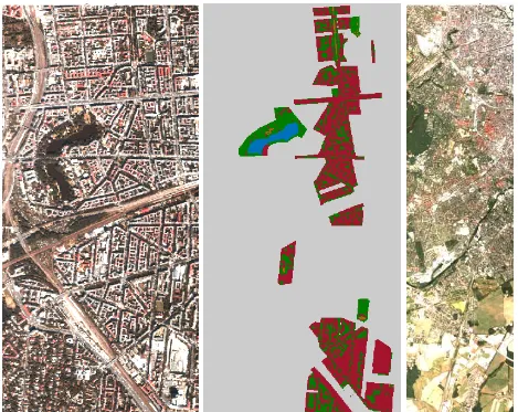
Our studies are performed using the Berlin-Urban-Gradient dataset Okujeni et al. (2016a), illustrated in Fig. 1. The dataset consists of a hyperspectral image, a simulated EnMAP scene, a manually derived spectral library, reference land cover informa-tion and reference fracinforma-tions for evaluainforma-tion.
3.1.1 HyMap Data The hyperspectral image was acquired from the Hyperspectral Mapper (HyMap), and serve as basis for the extracting of the archetypes. The study site is the South-west of Berlin, Germany, with a spatial resolution of3.6m. The HyMap image consists of 126 spectral bands, however, 15 noisy bands were removed resulting in 111 bands used for this work. The observed wavelengths are ranging from 0.45µm to 2.5µm, showing a high spectral information diversity, which enables a detailed analysis of the urban structure. In addition to the HyMap image, a manually derived reference image containing112.690 reference pixel is provided with valuable spectra, each labeled with one of the four land cover classes:impervious surface, vegetation, soil and water. The reference information is manually obtained by using digital orthophotos and cadastral data.
3.1.2 Simulated EnMAP Data EnMAP is German hyper-spectral satellite mission, which will start not earlier than 2018, with a focus on earth environmental observations in a global scale. Based on the HyMap data, an EnMAP scene was simu-lated using EnMAP End-to-End Simulation tool (EeteS, Segl et al. (2012)). The spatial resolution of30m is lower than the res-olution of the HyMap scene, and thus the mixing of land cover classes are more apparent. Just as the HyMap data EnMAP has a spectral resolution from0.45µm to2.5µm. For evaluation pur-poses,1495EnMAP pixels were obtained from the the simulation tool, containing the fractions of the land cover classes ranging from0to100%.
3.1.3 Manually Designed Spectral Library The spectral li-brary is a manually designed collection of75pure spectra ob-tained from the HyMap image. The spectra contain different land cover classes with39impervious surface spectra (different types of roof, pavement, tartan, pool water),31vegetation spec-tra (grass, tree),4soil spectra (uncovered ground, sand) and one natural water spectrum. All together, it is a balanced library for urban structures with39impervious and36pervious spectra. All spectra in the library can be assigned to a hierarchical urban clas-sification scheme, which was developed by Heiden et al. (2007). First, an initial collection of300spectra was selected by expert knowledge. Afterwards a two-step filtering was performed, in which the variability between the spectra is maximized in consid-eration of spectral variability of materials, brightness and shading
(a) Part of HyMap image data visualized as RGB-image with the wavelengths R =640nm, G =540nm and B = 450nm
(b) Reference image with four classes impervious surface(red),vegetation(green),soil(brown) and water(blue)
(c) Simulated EnMAP data vi-sualized with the wavelengths as specified above (bands: RGB = 11,5,1)
Figure 1. Berlin-Urban-Gradient dataset
effects. Moreover, in an iterative process those spectra for the fi-nal subset were selected that best describes the spectral diversity in a specific neighborhood. More details can be found in Okujeni et al. (2016a).
Experimental Setup
In our experiments the simulated EnMAP data is reconstructed by sparse representation using (1) the manually designed spec-tral library and (2) the automatically derived set of archetypes. The aim of the experiments is to show the suitability of the spec-tral libraries for sub-pixel quantification. Moreover, the goal is to show that the set of archetypes achieves a similar good or a bet-ter result than the manually designed spectral library. The sub-pixel quantification is evaluated with the given reference mixing fractions. Additionally, the number of used archetypes is evalu-ated and discussed. For this, two different sets of archetypes are used. The first setA1, contains all archetypes, extracted as pre-sented in the previous section. The second setA2, contains50% of all archetypes inA1, comprising only the archetypes with the smallest distance to the class-specific mean. Using the second set, we simulate datasets, which do not have a great variability in the feature space resulting in less archetypes. In summary,
three different dictionaries, namelyAA-R(usingA1andA2) and the manually designed spectral libraryLibare used for sub-pixel quantification with sparse representation. In order to guarantee an extraction of valuable archetypes, which are no outliers, the local outlier factor is applied, using10neighbors and a quantile of0.8as threshold on the pairwise distances.
Evaluation
For evaluation, several statistics are provided. First, the recon-struction error of the sparse representation is provided, indicating the ability of the elementary spectra to represent the EnMAP pix-els. Moreover, the result of the sparse representation is evaluated by a comparison between reference and actual estimated fraction coefficients. In this way, a measure is provided to evaluate the as-signments to the correct land cover class. This is done by means of the overall and class-wise mean absolute error (MAE) between reference and actual coefficients.
MAE = 1
S
S X
i=1
|(αi−αs)|, (5)
Table 1. Overall () and class-wiseMAE, reconstruction errorkγk2, and class-wise sum over all fractions based on the sub-pixel quantification of the EnMAP reference data. In the first two rows are the results for the archetypal reconstruction using a different number of archetypes (40 and 20) contained in the setA1and the setA2, denoted byAA-R. The last row contains the results for the
reconstruction using the manually designed spectral library (Lib) with all contained spectra (75). Bold numbers indicate the best results.
Amount kγk2 class-wise MAE [%] MAE [%] coefficient sum over all pixel
imp. surface vegetation soil water imp. surface vegetation soil water
AA-R 40 1,1 12,2 11,0 2,5 1,9 6,8 766,2 669,2 21,3 36,8
AA-R 20 1,2 13,6 10,8 1,8 6,1 8,1 658,1 704,9 17,8 112,2
Lib 75 0,0 16,0 9,2 2,1 12,2 9,9 556,9 695,4 32,0 208,8
True values of EnMAP data 754,8 674,4 27,0 36,8
smaller the MAE, the better the reconstruction by sparse rep-resentation. Moreover, the class-wise sum of the class fractions is provided.
Results and Discussion
3.4.1 Archetypal Analysis The total number and the quality of the archetypes have a significant influence on the success of the sparse representation. In theory, it is generally not known be-forehand how many archetypes can be generated from the data. It depends primarily on the data dimension and the inner variability of the data distribution. In our experiments, the archetypes are extracted from the given reference image (see Sec. 3.1.1), which is previously outlier-cleaned as specified in Sec. 3.2.
Given the data, the number of extracted archetypes in setA1 is40and the number in setA2 is20, which both serve as ele-mentary spectra included in the dictionaryD. The first archetype setA1 consists of25impervious surface spectra,12vegetation spectra,2soil spectra and one water spectrum. Except the water spectrum, the amount is class-wise halved (12 impervious surface spectra, 6 vegetation spectra, 1 soil spectra, 1 water spectrum) to create the second setA2. We observed that an extraction of more than40archetypes means that some archetypes lie in the center of the datasetX. The reason for this is that from a certain point on, positions in the center ofXhave the maximal distance to the previously extracted archetypes.
3.4.2 Sub-pixel Quantification Table 1 presents the results of the EnMAP sub-pixel quantification. TheMAEshows that all three dictionaries achieve a similar and satisfactory solution. The archetypes have a smaller class-wiseMAEforimpervious surfaceandwater, whereas the spectral library has a better re-sult forvegetation. Soilis reconstructed with a lowMAE by all approaches. However, the averageMAEobtained from both archetypal sets is better (7% and 8%) than from the spec-tral library (10%), even though there are more elementary spectra used for sub-pixel quantification. We assume that some entries in the spectral library are less helpful, because they are either not representative enough, or they do not fit to the observed pixel, or they do not contain additional information with respect to the other spectra. However, the high number of elementary spectra results in a small reconstruction error. On the right side of Ta-ble 1 we provide the coefficient sum over all pixel. Compared to the true values of EnMAP data, the reconstruction using setA1 leads to the smallest differences in the classesimp. surface, vegetationandwater. With respect to our goal to quantify the sub-pixel fractions there is no direct relation to theMAE. It is possible to obtain a correct coefficient sum and aMAE, even if
the amount of under- and overestimated fractions is large, exactly when the fractions are in equal share.
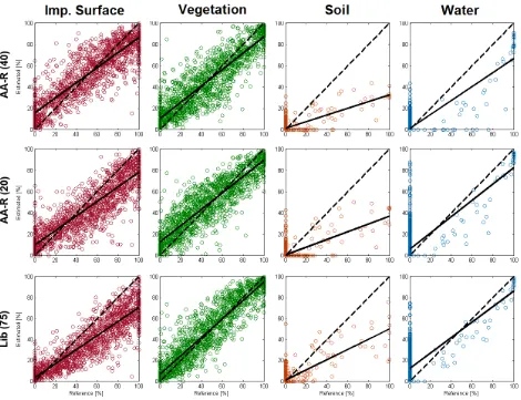
Figure 2 shows the class-wise fraction estimates, opposed to the reference fractions. There are1495dots in each plot. It can be observed that soil and water have a high proportion of0% reference fractions and lesser>0%fractions thanimpervious surfaceandvegetation. Theimpervious surfacescatter plot show that forAA-R-40the two lines intersect nearly the 55% point on the x-axis. This means that the estimated fractions are usually too high for all pixels which have a degree of impervi-ous surfaces over55%, and otherwise too small for smaller val-ues than the intersection point. In comparison toAA-R-20and Lib, where the reference values are mostly underestimated, the first set of archetypesA1shows the best result forimpervious surface. Thevegetationscatter plots do not have large dis-crepancies between the true 1:1 line (dashed line) and the esti-mated least-squares regression line (solid line), and the obtained results are similar for all used sets of elementary spectra. Addi-tionally, the scatter plots forsoillook similar, but overall not as good as for the other three classes. As specified above there is a high amount of0%fractions, which are estimated with up to 30%when using theAA-R-40spectra andLiband40%fractions when usingAA-R-20spectra. Furthermore, all pixels withsoil -fractions are clearly underestimated equally. We assume that the small number of elementary spectra is insufficient for the spec-tral diversity ofsoilpixels. Finally, the described observation with high estimated0%fractions also occurs in the water class with values over90%(AA-R-20). This is more apparent forLib andAA-R-20than forAA-R-40. However, the underestimation of the remaining pixels is smaller inLibthan inAA-R-40and AA-R-20.
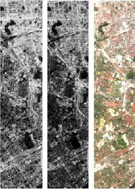
Figure 4 shows the degree of imperviousness in an exemplarily part of the EnMAP scene. The fraction map of theimpervious surfaceis visualized as gray value image. It is apparent that the left fraction map, derived byAA-R-40, is much brighter than this one obtained byLib. Thus, the degree of imperviousness of50.6%forAA-R-40is higher than35.1%forLib. Despite the fact that the actual degree of imperviousness is not given for this part from Berlin, the sum of all fractions is given for the reference pixels in Table 1 and can be used for comparison. The reference value of754,8forimpervious surfaceis slightly overestimated byAA-R-40, but clearly underestimated by 200 by Lib.
Figure 3 illustrates how often each spectrum is used for recon-struction for the determination of the fractions in1493EnMAP pixels.AA-R-40shows that there are significant elementary spec-tra, e.g., 10, 29 and 31, which often have a high fraction in the
Figure 2. Scatter plots representing the class-wise fraction estimates ofimpervious surface,vegetation,soilandwater, opposed to the reference fractions. A correct estimated pixel lies on the dashed line. The solid line represents the respective
least-square regression line for the scatter points.
reconstruction. In the other side, there are some elementary spec-tra in all plots which are used rarely. In can be observed that there is generally no dependence between the height of a bar, i.e. the number of non-zero estimated fractions for the spectra, and its overall fraction’s sum for all pixels. A striking example is spectra 3 in theAA-R-40plot. It is used for more than1200pixel recon-structions, but its fraction’s sum is only one third in comparison to spectra 10, which shows a similar high amount of uses. Espe-cially noticeable are the differences in the bar for the classwater between the manually designed library and the archetypes. A water spectrum has the special characteristic that there are only small reflectance values over all bands, so that it acts almost as a linear factor. Because of this, it is well suited to support all re-constructions, resulting in a high overall fraction sum. Its value in the manually designed spectral library is high with a fraction’s sum over200, in comparison toAA-R-40which shows a sum of fractions identical to the true value (see Table 1). ForAA-R-20 the sum of water fractions is higher than forAA-R-40. We as-sume the reason for this is the less number of elementary spectra, where oftentimes a reconstruction with water spectra is helpful regardless of the presence of water in the pixel.
We can also compare our results to Rosentreter et al. (2017), who use more sophisticated classification and regression techniques to reconstruct the EnMAP data with the same spectral libraryLib. When using Import or Support Vector Machines the overallMAE
(8,65% and10,22%) is slightly worse thanAA-R. Similar re-sults yield the regression techniques Support Vector Regression (10,06%) and Multioutput Support Vector Regression (6,92%). The computing time is many hours in contrast to a few minutes in this work. Considering the computational cost of those ap-proaches the quality of our results is remarkable.
CONCLUSION
Figure 3. The figure shows how often a elementary spectra is used for reconstruction of the reference EnMAP pixels. The maximal possible height of a bar is1493, if the elementary spectrum would be involved in the reconstruction of all reference EnMAP pixels.
The grew parts specify the sum of the fractions (i.e., the estimated coefficients) over all pixel.
more elementary spectra. Moreover the class-wise results shows mostly a good estimation of class fractions forimp. surface andvegetation, but an underestimation forsoilandwaterfor all used libraries.
In summary, the automatically extracted archetypal spectral brary is an adequate alternative to a manually derived spectral li-brary. In case no reference data is given, the interpretation can be done in a fast way by assigning land cover classes to the extracted archetypes using expert knowledge. The presented approach can also by combined with spatial information, which may further increase the approximation ability and accuracy of the fraction estimates. A worthwhile direction of further investigations is the combination of archetypal analysis with more sophisticated mod-els for sub-pixel quantification.
ACKNOWLEDGEMENTS
The authors would like to thank Akpona Okujeni, Sebastian van der Linden and Patrick Hostert for providing the dataset. More-over, the authors would like to thank Johannes Rosentreter for valuable discussions.
References
Bioucas-Dias, J. M., Plaza, A., Dobigeon, N., Parente, M., Du, Q., Gader, P. and Chanussot, J., 2012. Hyperspectral unmixing overview: Geometrical, statistical, and sparse regression-based approaches.IEEE Journal of Selected Topics in Applied Earth Observations and Remote Sensing5(2), pp. 354–379.
Breunig, M. M., Kriegel, H.-P., Ng, R. T. and Sander, J., 2000. Lof: Identifying density-based local outliers. SIGMOD Rec. 29(2), pp. 93–104.
Chan, T.-H., Ma, W.-K., Ambikapathi, A. and Chi, C.-Y., 2011. A simplex volume maximization framework for hyperspectral endmember extraction.IEEE Transactions on Geoscience and Remote Sensing49(11), pp. 4177–4193.
Craig, M. D., 1994. Minimum-volume transforms for remotely sensed data. IEEE Transactions on Geoscience and Remote Sensing32(3), pp. 542–552.
Cutler, A. and Breiman, L., 1994. Archetypal analysis. Techno-metrics36(4), pp. 338–347.
Guanter, L., Kaufmann, H., Segl, K., Foerster, S., Rogass, C., Chabrillat, S., Kuester, T., Hollstein, A., Rossner, G., Chlebek,
Figure 4. Fraction maps ofimpervious surfacein an exemplarily part of the EnMAP scene to estimate the degree of
imperviousness derived byAA-R-40(left) andLib(middle). The pixel-wise degree of imperviousness lies between 0%
(black) and 100% (white). The right image shows the corresponding EnMAP-scene is plotted (RGB = 11,5,1).
C. et al., 2015. The enmap spaceborne imaging spectroscopy mission for earth observation.Remote Sensing7(7), pp. 8830– 8857.
Heiden, U., Segl, K., Roessner, S. and Kaufmann, H., 2007. De-termination of robust spectral features for identification of ur-ban surface materials in hyperspectral remote sensing data. Re-mote Sensing of Environment111(4), pp. 537–552.
Huang, X., Lu, Q. and Zhang, L., 2014. A multi-index learning approach for classification of high-resolution remotely sensed images over urban areas. ISPRS Journal of Photogrammetry and Remote Sensing90, pp. 36–48.
Mørup, M. and Hansen, L. K., 2012. Archetypal analysis for ma-chine learning and data mining. Neurocomputing80, pp. 54– 63.
Okujeni, A., van der Linden, S. and Hostert, P., 2016a. Berlin-urban-gradient dataset 2009 - an enmap preparatory flight cam-paign (datasets). GFZ Data Services.
Okujeni, A., van der Linden, S., Suess, S. and Hostert, P., 2016b. Ensemble learning from synthetically mixed training data for quantifying urban land cover with support vector regression. IEEE Journal of Selected Topics in Applied Earth Observa-tions and Remote Sensing.
Plaza, A., Mart´ınez, P., P´erez, R. and Plaza, J., 2004. A quan-titative and comparative analysis of endmember extraction
al-gorithms from hyperspectral data. IEEE transactions on geo-science and remote sensing42(3), pp. 650–663.
Powell, R. L., Roberts, D. A., Dennison, P. E. and Hess, L. L., 2007. Sub-pixel mapping of urban land cover using multiple endmember spectral mixture analysis: Manaus, brazil.Remote Sensing of Environment106(2), pp. 253–267.
Priem, F., Okujeni, A., van der Linden, S. and Canters, F., 2016. Use of multispectral satellite imagery and hyperspec-tral endmember libraries for urban land cover mapping at the metropolitan scale. In: SPIE Remote Sensing, International Society for Optics and Photonics.
Roessner, S., Segl, K., Bochow, M., Heiden, U., Heldens, W. and Kaufmann, H., 2011. Potential of hyperspectral remote sensing for analyzing the urban environment. Urban remote sensing: Monitoring, synthesis and modeling in the urban environment pp. 49–61.
Rosentreter, J., Hagensieker, R., Okujeni, A., Roscher, R. and Waske, B., 2017. Sub-pixel mapping of urban areas using enmap data and multioutput support vector regression. IEEE Journal of Selected Topics in Applied Earth Observations and Remote Sensing. to appear.
Segl, K., Guanter, L., Rogass, C., Kuester, T., Roessner, S., Kauf-mann, H., Sang, B., Mogulsky, V. and Hofer, S., 2012. Eetes-the enmap end-to-end simulation tool. IEEE Journal of Se-lected Topics in Applied Earth Observations and Remote Sens-ing5(2), pp. 522–530.
Somers, B., Asner, G. P., Tits, L. and Coppin, P., 2011. Endmem-ber variability in spectral mixture analysis: A review. Remote Sensing of Environment115(7), pp. 1603–1616.
Suess, S., van der Linden, S., Leitao, P. J., Okujeni, A., Waske, B. and Hostert, P., 2014. Import vector machines for quantitative analysis of hyperspectral data. IEEE Geoscience and Remote Sensing Letters11(2), pp. 449–453.
Thurau, C., Kersting, K. and Bauckhage, C., 2010. Yes we can: simplex volume maximization for descriptive web-scale matrix factorization. In: Proceedings of the 19th ACM international conference on Information and knowledge management, ACM, pp. 1785–1788.
Veganzones, M. A. and Grana, M., 2008. Endmember extrac-tion methods: A short review. In:International Conference on Knowledge-Based and Intelligent Information and Engineer-ing Systems, Springer, pp. 400–407.
Wang, R., Li, H., Liao, W. and Huang, X., 2016. Endmember initialization method for hyperspectral data unmixing.Journal of Applied Remote Sensing10(4), pp. 042009.
Weng, Q., 2012. Remote sensing of impervious surfaces in the urban areas: Requirements, methods, and trends.Remote Sens-ing of Environment117, pp. 34–49.
Zhao, C., Zhao, G. and Jia, X., 2017. Hyperspectral image un-mixing based on fast kernel archetypal analysis.IEEE Journal of Selected Topics in Applied Earth Observations and Remote Sensing10(1), pp. 331–346.
Zhao, G., Zhao, C. and Jia, X., 2016. Multilayer unmixing for hy-perspectral imagery with fast kernel archetypal analysis.IEEE Geoscience and Remote Sensing Letters 13(10), pp. 1532– 1536.