SPATIAL-SPECTRAL CLASSIFICATION BASED ON THE UNSUPERVISED
CONVOLUTIONAL SPARSE AUTO-ENCODER FOR HYPERSPECTRAL REMOTE
SENSING IMAGERY
Xiaobing Han a,b, Yanfei Zhong a,b, *, Liangpei Zhang a,b
a State Key Laboratory of Information Engineering in Surveying, Mapping and Remote Sensing, Wuhan University, Wuhan 430079,
China
b Collaborative Innovation Center of Geospatial Technology, Wuhan University, Wuhan 430079, China
Commission VII, WG VII/3
KEY WORDS: spatial-spectral classification, hyperspectral remote sensing imagery, sparse auto-encoder (SAE), convolution, unsupervised convolutional sparse auto-encoder (UCSAE)
ABSTRACT:
Current hyperspectral remote sensing imagery spatial-spectral classification methods mainly consider concatenating the spectral information vectors and spatial information vectors together. However, the combined spatial-spectral information vectors may cause information loss and concatenation deficiency for the classification task. To efficiently represent the spatial-spectral feature information around the central pixel within a neighbourhood window, the unsupervised convolutional sparse auto-encoder (UCSAE) with window-in-window selection strategy is proposed in this paper. Window-in-window selection strategy selects the sub-window spatial-spectral information for the spatial-spectral feature learning and extraction with the sparse auto-encoder (SAE). Convolution mechanism is applied after the SAE feature extraction stage with the SAE features upon the larger outer window. The UCSAE algorithm was validated by two common hyperspectral imagery (HSI) datasets—Pavia University dataset and the Kennedy Space Centre (KSC) dataset, which shows an improvement over the traditional hyperspectral spatial-spectral classification methods.
* Corresponding author
1. INTRODUCTION
During the past 30 years, the airborne or space-borne imaging spectrometer has been rapidly developed, which helps gather a huge amount of hyperspectral imagery data with hundreds of bands covering a broad spectrum of wavelength range. It is noted that the hyperspectral imagery contains rich spectral information and has proven to be effective for discriminating the ground objects. Meanwhile, with the development of the sensors, the hyperspectral imaging techniques can also provide abundant detail and structural spatial information (Grahn et al., 2007, Camps-Valls et al., 2014, Landgrebe et al., 2003, Zhao et al., 2015a, Zhao et al., 2015b). The high spectral resolution and high spatial resolution properties enable the hyperspectral imagery data to become very useful and widely applicable in agriculture, surveillance, astronomy, mineralogy, and environment science areas (Chang et al., 2013, Fauvel et al., 2013, Feng et al., 2016, Jiao et al., 2015, Zhong et al., 2012). Among the various application areas, the most common utilization of the hyperspectral imagery data is the ground object classification.
The traditional ground object classification tasks from the hyperspectral imagery data are mainly solved by exhaustively considering the spectral signatures. However, current hyperspectral imagery data can provide both rich spectral information and finer spatial information, which increases the possibilities of more accurately discriminating the ground objects. Therefore, finding an effective manner of efficiently exploiting both the spectral information and the neighbourhood spatial information around the central pixel from the hyperspectral imagery is of great significance (Zhou et al., 2015, Ji et al., 2014, Kang et al., 2014, Jimenez et al., 2005). Various spatial-spectral feature classification methods have been
proposed, including the neighbourhood window opening operations (Chen et al., 2014, Plaza et al., 2009), morphological operations (Fauvel et al, 2008), and segmentation approaches. All these spatial-spectral feature classification methods focus on combining the spectral information vectors and the spatial information vectors together into a long vector, and the common characteristics of these algorithms can be categorized as spatially constrained approaches. These methods mainly consider the spectral information and the spatial information in a separate manner, and cause the spectral and spatial information loss and connection deficiency. When given a fixed larger spatial neighbourhood window around the central pixel, how to exhaustively extract the information within the larger outer window is a critical problem to be solved. In recent years, Deep learning (Hinton and Salakhutdinov, 2006, Hinon et al., 2006, Bengio et al., 2007) has developed very fast and achieved great success due to its powerful feature extraction and feature representation ability. Deep learning consists of two types of feature extraction and feature representation models— supervised feature learning models and unsupervised feature learning models. Among the unsupervised feature learning models, sparse auto-encoder (SAE) (Ng et al., 2010) is a kind of efficient feature extraction method, which adopts the reconstruction-oriented feature learning manner. Finding an efficient feature representation approach is at the core of the hyperspectral imagery spatial-spectral feature classification task. To better represent the spatial-spectral information from the hyperspectral imagery, SAE is exploited in this paper due to its specific feature extraction ability and automatic and integrated spatial and spectral information representation manner.
To cooperate with the high spectral and finer spatial properties from the hyperspectral imagery, SAE is exploited with the window-in-window selection strategy to better ISPRS Annals of the Photogrammetry, Remote Sensing and Spatial Information Sciences, Volume III-7, 2016
represent the spatial and spectral information around the central pixel. Similar to the heterogeneous property consideration of the conventional neighbourhood window opening operation, window-in-window selection strategy works by first selecting a larger outer window around the central pixel and then by stochastically selecting the sub-windows within this larger outer window. SAE is utilized for extracting the features from these sub-windows, which helps produce a set of representative SAE features. Throughout the SAE feature extraction, a deeper-level intrinsic features within a certain local spatial window are extracted.
After the SAE feature extraction, the SAE features contain abundant orientation and structural information. To fully utilize the SAE features upon the larger outer windows, an effective convolution mechanism is utilized. After convolution, the convolved feature maps are the response sets containing each of the SAE feature responding to the larger outer window, which conserve abundant detail and structural information for the larger outer windows. Throughout the UCSAE algorithm classification process, a deeper-level of spatial-spectral feature classification for the hyperspectral imagery is performed.
In this paper, the UCSAE has two specific contributions. Firstly, this paper first adopts the window-in-window local spatial-spectral information selection strategy, which facilities the local SAE feature extraction on the sub-windows. Secondly, this paper first applies the convolution mechanism to represent the spatial-spectral features for the hyperspectral imager classification task, which generates the feature responses of the SAE features upon the lager outer windows and helps conserve the information responses to the maximum extent.
The rest of this paper is organized as follows. Section II mainly introduces the deep learning related works. Section III explicitly explains the main hyperspectral spatial-spectral feature classification algorithm--the unsupervised convolutional sparse auto-encoder (UCSAE). In section IV, the experimental results conducted with the UCSAE algorithm on two widely utilized hyperspectral imagery datasets are presented and the experimental analysis is given in detail. The final section concludes the proposed algorithm for hyperspectral imagery spatial-spectral classification.
2. DEEP LEARNIING RELATED WORKS
Deep learning (Hinton and Salakhutdinov, 2006, Hinton et al., 2006, Begnio et al., 2007, Ng et al., 2010, Simard et al., 2003, Krizhevsky et al., 2012, Bengio et al., 2009, Boureau et al., 2010, LeCun et al., 1998) is another development of the machine learning areas by solving the limited feature expression ability from the conventional machine learning techniques with more deep layers to automatically extract the features from the original images. According to the paper (LeCun et al.,2015), deep learning allows computational models composed of multiple processing layers to learn representations of data with multiple levels of abstraction, meaning that deep learning discovers the intricate structures in large datasets by utilizing the backpropagation algorithm to indicate how a machine should change it internal parameters.
It is noted that deep learning can be divided into two categories—supervised feature learning and unsupervised feature learning. Supervised feature learning is the most common form of machine learning, whether the network structure is deep or not. Supervised feature learning tries to compute an objective function that measures the error between the output scores and the desired pattern of scores. Through modifying the internal adjustable parameters with backpropagation algorithm and the chain rules, the error of the
supervised feature learning is reduced. For supervised feature learning, these adjustable parameters usually are the network weights to be adjusted. The difference between the supervised feature learning and the unsupervised feature learning is that supervised feature learning optimizes the network weights by considering the supervised label information into the network, while unsupervised feature learning creates layers of feature detectors without requiring labelled data. The objective of unsupervised feature learning is that each layer of the feature detectors was to be able to reconstruct or model the activities of feature detectors in the layer below. However, both the supervised feature learning and the unsupervised feature learning can be regarded as constructed from multiple simple building blocks, which can transform the low-level feature representation into the high-level feature representation. In recent years, various deep learning models were studied, including convolutional neural networks (CNN) (Simard et al., 2003), deep belief networks (DBN) (Hinton et al., 2006, Bengio et al., 2007), auto-encoder (AE) (Hinton and Salakhutdinov, 2006), denoising auto-encoder (DAE) (Vincent et al., 2008a, Vincent et al., 2010b), and the reconstruction-oriented sparse auto-encoder (SAE).
SAE is an efficient unsupervised reconstruction-oriented feature extraction model, which optimizes the network weights by minimizing the network reconstruction error between the input data and the reconstructed data. The reason why the SAE can realize the goal of data reconstruction is that the hidden network reconstruction error with L-BFGS algorithm. The sparse property of the SAE is performed by adding the sparse constraint on the hidden units with Kullback-Leibler (KL) divergence, where the sparsity is measured between the given sparse value and the average value of the hidden unit activation. When these two values are close to the threshold, the value of the KL-divergence is set to 1, otherwise to 0. For SAE, when the input data of the SAE are local patches, the network can extract the representative local features. SAE also has an advantage of taking the whole dimensional information into consideration to reduce the information loss.
3. HYPERSPECTRAL IMAGERY SPATIAL-SPECTRAL CLASSIFICATION BASED ON THE UNSUPERVISED CONVOLUTIONAL SPARSE
AUTO-ENCODER
In this paper, the UCSAE algorithm has been proposed for the hyperspectral imagery spatial-spectral feature classification. Based on the accurate spectral signatures and abundant finer spatial information, how to adequately utilize the spectral and spatial information of the hyperspectral imagery is critical. Conventional spatial-spectral classification models are proposed by considering the spatial and spectral information separately or in a direct combination manner. Given a fixed window around the central pixel, in order to solve the connection deficiency problem between the spatial information and the spectral information, the SAE model in deep learning research fields was introduced in this paper with the window-in-window selection strategy. By learning the features within the larger outer window, the local features of the larger outer window can be obtained. To better represent the larger outer window with the SAE features, the convolution mechanism is introduced. The unsupervised convolutional sparse auto-encoder (UCSAE) ISPRS Annals of the Photogrammetry, Remote Sensing and Spatial Information Sciences, Volume III-7, 2016
introduced in this paper can be separated into three stages: 1) the SAE feature extraction with the window-in-window spatial-spectral information selection strategy; 2) spatial-spatial-spectral feature representation based on the convolution mechanism; and 3) spatial-spectral feature softmax classification. The follow part will show how each stage works.
3.1 SAE Feature Extraction with the Window-in-Window Spatial-Spectral Information Selection Strategy
The window-in-window spatial-spectral information selection strategy works in two steps. In the first step, the large outer spatial neighbourhood window around the central pixel was selected both considering the spectral information and the spatial neighbourhood information from the hyperspectral imagery. In the second step, the sub-windows needed are stochastically sampled within this larger outer window to extract the features via SAE. Given the larger outer window size around the central pixel isw w , the size of the sub-window isw1w1, the band number of the hyperspectral imagery isN, and the number of the sub-windows isM , then the direct concatenated spatial-spectral information vector is w1 w1 N M . To extract the features from the sub-windows around the central pixel from the hyperspectral imagery, the concatenated spatial-spectral information vectorw1 w1 N M will be imported into the sparse auto-encoder.
SAE is a reconstruction-oriented feature extraction model, which mines the intrinsic features of the sub-windows from the larger outer windows. Suppose that the sub-window sets input data are mapped into the hidden units; the decoding stage maps the hidden units into the reconstructed data. The hidden unit representation are shown in (1) and (2).
1 1 mapped into the reconstructed data in (3).
2 2 encoding weight and the decoding weight respectively;
1 K
bR and 2
N
b R are the biases respectively. For SAE, the network realizes the reconstruction process with tied weights 1 2
T
WW . After the SAE feature extraction procedure,
the features are transformed through : N K
f R R , where K is equal to the hidden unit number.
To better extract the features from the local sub-windows, the cost function of SAE is shown in (4), which is optimized with
In (4),Xand Zrepresent the input data and the reconstructed data, respectively. mis the number of samples for training; and represents the weight decay parameter;
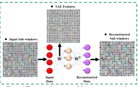
represents the sparse constraint coefficient. The third term in (4) represents the sparse term, where the sparse constraint is added with the KLdivergence. Figure 1 shows the network structure of the sparse auto-encoder.
Figure 1 The network structure of the sparse auto-encoder
3.2 Spatial-Spectral Feature Representation Based on the Convolution Mechanism
After the SAE feature extraction, the SAE features contain abundant representative detail and structural information of the
sub-windows from all of the pixels’ larger outer windows. The
SAE features are the representative features for all the categories. According to the convolution response mechanism, the convolved feature maps can fully represent the larger outer windows by calculating each of the SAE features with the larger outer window. Suppose that the size of the larger outer window is w w with N bands, the size of the SAE features is
1 1
ww with K channels. After convolution, the convolved feature map size for each of the larger outer window around the central pixel is (w w1 1) (w w1 1) Kwith the stride 1. After the convolution stage, the max pooling (Scherer et al., 2010) is added on the convolved feature maps.
3.3 Spatial-Spectral Feature Softmax Classification
After the convolution stage and the pooling stage, the pooled feature maps will be imported into the softmax classifier, where the size of the pooled feature maps is
1 1
((w w 1) / ) ((s w w 1) / )s K with pooling sizes. To classify each pixel, the softmax regression classifier is shown in (5). works step by step are introduced. To have a direct recognition of the UCSAE working mechanism, Figure 2 shows the detailed flowchart of the UCSAE algorithm.
Figure 2 The flowchart of UCSAE ISPRS Annals of the Photogrammetry, Remote Sensing and Spatial Information Sciences, Volume III-7, 2016
4. EXPERIMENTS AND ANALYSIS
In this section, we validated the proposed algorithm--UCSAE with two popular hyperspectral imagery datasets and presented the experimental results which demonstrates the benefits of UCSAE over the traditional hyperspectral imagery spatial-spectral feature classification methods—RBF-SVM (Chen et al., 2014), RBF-EMP (Fauvel et al., 2008), and SAE-LR (Chen et al., 2014). To evaluate the classification results by the UCSAE, the qualitative and quantitative evaluations are made, where the quantitative evaluation is measured by the overall classification (OA), average accuracy (AA), and the kappa coefficient criterions.
4.1 Experimental Hyperspectral Data Set Description
In the experimental part, two hyperspectral remote sensing imagery datasets were utilized to measure the UCSAE spatial-spectral classification performance. The first hyperspatial-spectral imagery dataset is the Pavia University dataset, and the second is the Kennedy Space Centre (KSC) dataset. The Pavia University dataset was gathered by the Reflective Optics System Imaging Spectrometer (ROSIS-3) sensor over the city of Pavia, Italy, with 610 340 pixels. This dataset contains 115 bands in the 0.43 0.86 m range of the electromagnetic spectrum, with a spatial resolution of 1.3 m per pixel. After removing some bands contaminated by noise, the remaining 103 bands were utilized for the final classification. For the Pavia University dataset, the 50% of the ground truth samples were stochastically selected as the training samples and the remaining samples were set as the test samples. The Pavia University image and the ground truth samples are shown in Figure 3, respectively. The training and testing sample settings were listed in Table.1. For the Pavia University dataset, the large outer window size is set as 7 7 and the size of the sub-windows is set as 4 4 .
Asphalt
Meadows
Gravel
Trees
Metal_sheets
Bare_soil
Bitumen
Bricks
Shadows
(a) (b)
Figure 3 (a) The Pavia University image. (b) The ground-truth samples for the Pavia University image.
Class number
Class name
Training samples
Test samples
1 Asphalt 3328 3327
2 Meadows 9337 9336
3 Gravel 1062 1061
4 Trees 1544 1544
5 Metal_sheets 685 684
6 Bare_soil 2527 2526
7 Bitumen 677 677
8 Bricks 1853 1853
9 Shadows 487 492
Overall 21500 21500
Table 1 Land-cover classes and the number of pixels for the Pavia University dataset
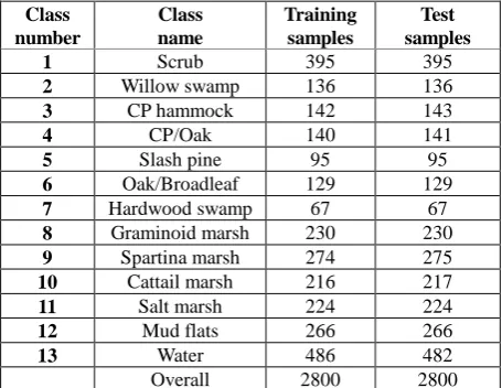
The second hyperspectral imagery dataset utilized for the experiment was the Kennedy Space Centre (KSC) dataset. The KSC dataset was acquired by the National Aeronautics and Space Administration (NASA) Airborne Visible/Infrared Imaging Spectrometer instrument (AVIRIS), which covers the electromagnetic spectrum range of 0.4 2.5 m with 224 bands, and consists of 512 614 pixels with a spatial resolution of 18 m. By removing the water absorption and low signal-to-noise ratio (SNR) bands, 176 bands were remained for the UCSAE spatial-spectral feature classification. For the KSC dataset, 50% of the training samples were set as the training samples, and the remaining samples were set as the test samples. The KSC image and the ground truth are shown in Figure 4. The training and testing sample setting are listed in Table 2. For the KSC dataset, the large outer window size is set as 7 7 and the size of the sub-windows is set as 4 4 .
Scrub
Willow swamp
CP hammock
CP/Oak
Slash pine
Oak/Broadleaf
Hardwood swamp
Graminoid marsh
Spartina marsh
Catiail marsh
Salt marsh
Mud flats
Water
Figure 4 The KSC image and the corresponding ground-truth samples.
Class number
Class name
Training samples
Test samples
1 Scrub 395 395
2 Willow swamp 136 136
3 CP hammock 142 143
4 CP/Oak 140 141
5 Slash pine 95 95
6 Oak/Broadleaf 129 129
7 Hardwood swamp 67 67
8 Graminoid marsh 230 230
9 Spartina marsh 274 275
10 Cattail marsh 216 217
11 Salt marsh 224 224
12 Mud flats 266 266
13 Water 486 482
Overall 2800 2800
Table 2 Land-cover classes and the number of pixels for the KSC dataset
4.2 Qualitative Evaluation of the UCSAE Based Spatial-Spectral Classification Results
For the Pavia University dataset, compared with RBF-SVM, EMP-SVM, and SAE-LR classification methods, the qualitative evaluation was shown in Figure 5.
(a) RBF-SVM (b) EMP-RBF
(c) SAE-LR (d) UCSAE
Figure 5 The classification maps for the different spatial-spectral classification methods.
From the classification maps in Figure 5, it can be seen that the classification results by UCSAE algorithm has a better classification result for the class of Bitumen. Comparing (a), (b), (c) and (d), it can be seen that (d) has better detail conservation in the overall view.
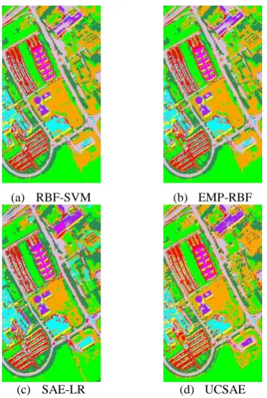
(a) RBF-SVM (b) EMP-RBF
(c) SAE-LR (d) UCSAE
Figure 6 The classification maps for the different spatial-spectral classification methods.
For the KSC dataset, compared with RBF-SVM, EMP-SVM, and SAE-LR classification methods, the qualitative evaluation was shown in Figure 6. From Figure 6, it can be seen that the classes of Willow swamp, CP/Oak, Slash pine, and Oak/Broadleaf achieve a better detail classification results, while the classes of Spartina marsh by RBF-SVM, EMP-RBF, SAE-LR, and UCSAE show a similar visual effect.
4.3 Quantitative Evaluation of the UCSAE Based Spatial-Spectral Classification Results
To quantitative evaluate the classification results in Figure 5 and Figure 6 for the Pavia University dataset and the KSC dataset, respectively, the quantitative evaluations of the Pavia University dataset and the KSC dataset are shown in Table 3 and Table 4, respectively.
Methods
RBF-SVM
EMP-RBF
SAE-LR UCSAE
Ac
cu
ra
cy
Asphalt 0.9919 0.9907 0.9763 0.9901 Meadows 0.9989 0.9988 0.9885 0.9943 Gravel 0.9359 0.9303 0.9727 0.9642 Trees 0.9786 0.9773 0.9832 0.9845 Metal_
sheets
1.0000 1.0000 1.0000 1.0000
Bare_ soil
0.8880 0.8492 0.9272 0.9394
Bitumen 0.9705 0.9631 0.9380 0.9542 Bricks 0.9795 0.9773 0.9288 0.9752 Shadows 0.9980 0.9980 0.9939 0.9898
OA 0.9777 0.9721 0.9720 0.9824
AA 0.9712 0.9650 0.9676 0.9769
Kappa 0.9707 0.9634 0.9634 0.9766 Table 3 Different spatial-spectral classification accuracy comparisons on the Pavia University dataset
From Table 3, it can be seen that the UCSAE algorithm achieves a 98.24% OA better than the traditional spatial-spectral classification methods. From Table 3, it can be seen that the classes of Trees, and Bare_soil obtain a better producer classification accuracy than the RBF-SVM, EMP-RBF and SAE-LR algorithms, while the classes of Gravel obtains a better producer classification accuracy by the UCSAE than the RBF-SVM, EMP-RBF, and SAE-LR algorithms. The reason why the UCSAE algorithm can obtain a better classification result for the Bare_soil class is mainly due to the neat and wide-range distributions and the spectral properties of these two classes that are more easily extracted by the UCSAE algorithm.
Methods
RBF-SVM
EMP-RBF SAE-LR UCSAE
Ac
cu
ra
cy
Scrub 0.9873 0.9873 0.9949 0.9921 Willow
swamp
0.9926 0.9926 0.9853 1.0000
CP hammock
0.8881 0.8881 0.9790 0.9609
CP/Oak 0.7234 0.7163 0.7305 0.9127 Slash
pine
0.7684 0.7789 0.9053 1.0000
Oak/ Broadleaf
0.8837 0.8992 0.8450 0.9123
Hardwood swamp
0.9851 0.9851 0.9851 0.9615
Graminoid marsh
1.0000 1.0000 1.0000 0.9953
Spartina marsh
1.0000 1.0000 1.0000 1.0000
Cattail marsh
1.0000 1.0000 1.0000 1.0000
Salt marsh
1.0000 1.0000 1.0000 0.9952 ISPRS Annals of the Photogrammetry, Remote Sensing and Spatial Information Sciences, Volume III-7, 2016
Mud Table 4 Different spatial-spectral classification accuracy comparisons on the KSC dataset range distributions of these classes.
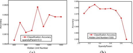
4.4 Parameter Analysis
Based on the theoretical explanation of the SAE, it’s noted that the hidden unit number and the sparsity are the main parameters influencing the classification properties. For the Pavia University dataset, according to (Coates et al., 2011), the optimal classification accuracy is obtained when the hidden unit number equals to 1000, and the sparsity value equals to 0.3. The parameter analysis for the Pavia University dataset is shown in Figure 7. sparsity parameter with the Pavia University dataset.
For the KSC dataset, the optimal classification accuracy is obtained when the hidden unit number is 1300 and the sparsity value is 0.5. The detailed parameter analysis is shown in Figure 8.
600 800 1000 1200 1400 1600 0.977 sparsity parameter with the KSC dataset.
5. CONCLUSIONS
Based on the feature extraction superiority of the SAE model and the efficient feature representation power by convolution mechanism, a novel spatial-spectral classification algorithm named UCSAE has been proposed for hyperspectral remote sensing imagery. Within a fixed spatial neighbourhood window around a central pixel, the UCSAE shows better classification
performance than the direct spatial-spectral classification methods due to its intrinsic feature extraction properties. To better extract the features within the larger outer windows, the window-in-window spatial-spectral information selection strategy is proposed in this paper for the latter SAE feature extraction procedure. As for the UCSAE algorithm, it can provide an information conservation manner in the classification procedure. The experimental results demonstrate that the proposed UCSAE algorithm can obtain a better spectral classification performance over the traditional spatial-spectral classification methods on the Pavia University dataset and the KSC dataset. Besides, when the experimental area is larger but with uniform ROI (area of interest) sampling on the imagery, this method is also applicable.
ACKNOWLEDGEMENTS
This work was supported by National Natural Science Foundation of China under Grant No. 41371344, State Key Laboratory of Earth Surface Processes and Resource Ecology under Grant No. 2015-KF-02, Program for Changjiang Scholars and Innovative Research Team in University under Grant No. IRT1278, Natural Science Foundation of Hubei Province under Grant No. 2015CFA002, and Open Research Fund Program of Shenzhen Key Laboratory of Spatial Smart Sensing and Greedy layer-wise training of deep networks. Adv. in Neur. In., vol. 19.
Boureau, Y.-L; Bach, F.; LeCun, Y.; Ponce, J., 2010. Learning mid-level features for recognition. In Proceedings of IEEE Conf.
Computer Vision and Pattern Recognition (CVPR), pp.2559–
2566.
Camps-Valls, G.; Tuia, D.; Bruzzone, L.; Benediktsson. J.A., 2014. Advances in hyperspectral image classification: Earth monitoring with statistical learning methods. IEEE Signal
Process. Mag, vol. 31, pp. 45-54.
Chang, C.-I., 2013. Hyperspectral data processing: algorithm design and analysis. John Wiley & Sons.
Chen, Y.; Lin, Zh.; Zhao, X.; Wang, G.; Gu, Y., 2014. Deep Learning-based Classification of Hyperspectral Data. IEEE J.
Sel. Topics Appl. Earth Observ. Remote Sens., vol. 7, pp.
2094-2107.
Coates, A.; Ng, A. Y.; Lee, H., 2011. An analysis of single-layer networks in unsupervised feature learning. In Proceedings of the International Conference on Artificial Intelligence and
Statistics, pp. 215–223.
Fauvel, M.; Benediktsson, J.A.; Chanussot, J.; Sveinsson, J.R., 2008. Spectral and spatial classification of hyperspectral data using SVMs and morphological profiles. IEEE Trans. Geosci.
Remote Sens., vol. 46, pp. 3804-3814.
Fauvel, M.; Tarabalka, Y.; Benediktsson, J.A.; Chanussot, J.; Tilton, J.C., 2013. Advances in spectral-spatial classification of hyperspectral images. Proceedings of IEEE, vol. 101, pp. 652-675.
Grahn, H. F; Geladi, P., 2007. Techniques and Applications of Hyperspectral Image Analysis. Hoboken, NJ, USA: Wiley. Hinton, G. E.; Osindero, S.; Y.-W, 2006. A fast learning algorithm for deep belief nets. Neural Comput., vol. 18, pp. 1527-1554.
Hinton, G. E.; Salakhutdinov, R.R., 2006. Reducing the dimensionality of data with neural networks. Science, vol. 313, pp. 504-506.
H. Jiao, Y. Zhong, and L. Zhang, 2012. "Artificial DNA computing-based spectral encoding and matching algorithm for hyperspectral remote sensing data," IEEE Transactions on
Geoscience and Remote Sensing, vol. 50, no. 10, pp. 4085-4104.
Ji, R.; Gao, Y.; Hong, R.; Liu, Q.; Tao, D.; Li, X., 2014. Spectral-Spatial Constraint Hyperspectral Image Classification.
IEEE Trans. Geosci. Remote Sens., vol. 52, pp. 1811-1824.
J. Zhao, Y. Zhong, and L. Zhang, 2015a. "Detail-Preserving Smoothing Classifier Based on Conditional Random Fields for High Spatial Resolution Remote Sensing Imagery," IEEE
Transactions on Geoscience and Remote Sensing, vol. 53, no. 5,
pp. 2440-2452.
J. Zhao, Y. Zhong, Y. Wu, L. Zhang, and H. Shu, 2015b. "Sub-pixel mapping based on conditional random fields for hyperspectral remote sensing imagery," IEEE Journal of
Selected Topics in Signal Processing, vol. 9, no. 6, pp.
1049-1060.
Jimenez, L. O.; Rivera-Median, J. L.; Rodirguez-Diaz, E., 2005. Integration of spatial and spectral information by means of unsupervised extraction and classification for homogenous objects applied to multispectral and hyperspectral data. IEEE
Trans. Geosci. Remote Sens., vol. 43, pp. 844-851.
Kang, X.; Li, Sh.; Benediktsson, J.A., 2014. Spectral-Spatial Hyperspectral Image Classification with Edge-Preserving Filtering. IEEE Trans. Geosci. Remote Sens., vol. 52, pp. 2666-2677.
Krizhevsky, A.; Sutskever, I.; Hinton, G., 2012. ImageNet classification with deep convolutional neural networks. In
Proceedings of Advances in Neural Information Processing
Systems (NIPS), vol. 25, pp. 1090–1098.
Landgrebe, D., 2003. Signal Theory Methods in Multispectral Remote Sensing. Hoboken, NJ, USA: Wiley.
LeCun, Y.; Bengio, Y.; Hinton, G.E., 2015. Deep Learning.
Nature, vol. 521, pp. 436-444.
LeCun, Y.; Bottou, L.; Bengio, Y.; Haffner, P., 1998. Gradient based learning applied to document recognition. Proceedings of IEEE, vol. 86, pp. 2278-2324.
Ng, Andrew, 2010. Sparse autoencoder. CS294A Lecture notes, Stanford Univ..
Plaza, A.; Plaza, J.; Martin, G., 2009. Incorporation of spatial constraints into spectral mixture analysis of remotely sensed hyperspectral data. In Proceedings of IEEE Int. Workshop
Machine Learning Signal Processing, pp. 1-6.
Boureau, Y.-L.; Bach, F., LeCun,Y.; Ponce, J., 2010. Learning mid-level features for recognition.
R. Feng, Y. Zhong, Y. Wu, X. Xu, D. He, and L. Zhang, 2016. "Nonlocal Total Variation Subpixel Mapping for Hyperspectral Remote Sensing Imagery," Remote Sensing, vol. 8, no. 3, p. 250. Simard, P. Y.; Steinkraus, D.; Platt, J. C., 2003. Best practices for convolutional neural networks applied to visual document analysis. Int. Conf. Document Analysis and Recognition, vol. 2, pp. 958–962.
Vincent, P.; Larochelle, H.; Bengio, Y.; Manzagol, P.-A., 2008a. Extracting and composing robust features with denoising auto-encoders. In Proceedings of ACM Int. Conf.
Machine Learning, pp. 1096-1103.
Vincent, P.; Larochelle, H.; Lajoie, I.; Bengio, Y.; Manzagol, P., 2010b. Stacked denoising autoencoders: Learning Useful Representations in a Deep Network with a Local Denoising Criterion. J. Mach. Learn. Res., vol. 11, pp. 3371-3408. Y. Zhong and L. Zhang, 2012. "An adaptive artificial immune network for supervised classification of multi-/hyperspectral
remote sensing imagery," IEEE Transactions on Geoscience
and Remote Sensing, vol. 50, no. 3, pp. 894-909.
Zhou, Y.; Wei, Y., 2015. Learning Hierarchical Spectral-Spectral Features for Hyperspectral Image Classification. IEEE Trans. Cybern..