Conference paper

(1)

RECONSTRUCTING 3D COASTAL CLIFFS FROM AIRBORNE OBLIQUE

PHOTOGRAPHS WITHOUT GROUND CONTROL POINTS

T.J.B. Dewez

BRGM – French Geological Survey, 45060 Orleans-la-Source, France – t.dewez@brgm.fr

Commission V

KEY WORDS: Oblique airborne photos, Structure-from-motion, georeferencing, ground control point, GPS, Normandy, cliff,

point cloud, Visual SFM

ABSTRACT:

Coastal cliff collapse hazard assessment requires measuring cliff face topography at regular intervals. Terrestrial laser scanner techniques have proven useful so far but are expensive to use either through purchasing the equipment or through survey subcontracting. In addition, terrestrial laser surveys take time which is sometimes incompatible with the time during with the beach is accessible at low-tide. By comparison, structure from motion techniques (SFM) are much less costly to implement, and if airborne, acquisition of several kilometers of coastline can be done in a matter of minutes. In this paper, the potential of GPS-tagged oblique airborne photographs and SFM techniques is examined to reconstruct chalk cliff dense 3D point clouds without Ground Control Points (GCP). The focus is put on comparing the relative 3D point of views reconstructed by Visual SFM with their synchronous Solmeta Geotagger Pro2 GPS locations using robust estimators. With a set of 568 oblique photos, shot from the open door of an airplane with a triplet of synchronized Nikon D7000, GPS and SFM-determined view point coordinates converge to X: ±31.5m; Y: ±39.7m; Z: ±13.0m (LE66). Uncertainty in GPS position affects the model scale, angular attitude of the reference frame (the shoreline ends up tilted by 2°) and absolute positioning. Ground Control Points cannot be avoided to orient such models.

1. INTRODUCTION

Geomorphology is concerned with determining the processes that shape landscapes. Repeated close-range measurements offer a way to observe and quantify these processes. Two technologies have emerged recently to capture surface topography with great detail: laser scanning (terrestrial and mobile)(among many others Rosser et al. 2005; Dewez et al. 2007, 2013; Lague et al. 2013) and structure-from-motion (SFM) (Ahmadabadian et al. 2013; James & Robson, 2011). SFM applications are expanding at growing speed because they rely on commonly available hardware: a camera. Processing can be done with widely available software such as Visual SFM at no cost if used for research purposes. To produce data of any value to geoscientists, however, SFM results need be precisely and accurately oriented in space, which is often done with Ground Control Points. Measuring these is time consuming and not always optimally distributed. In this piece of work, we examine if GCP can be done away with when combining SFM techniques with off-the-shelf digital SLR (Nikon D7000) equipped with third-party geotagging GPS device (Solmeta Geotagger Pro2, hardware v.3). We chose to shoot the photos through the open door of a parachuting plane because a lot of ground could be covered in little time. Typically, the entire 120km chalk coast of Normandy and Picardy was surveyed in less than 2 hours, meaning at nearly constant low-tide level, for a cost close to 2000€. The technical focus of the paper consists in solving the 7-parameter transform between 3D model coordinates and World GPS coordinates, accounting for gross GPS error contamination and assessing the coherence between GPS-measured and SFM-reconstructed camera viewpoints.

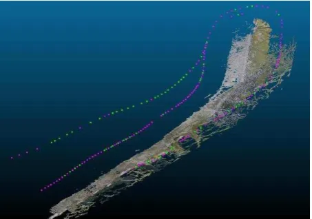
Figure 1 : 3D point cloud and camera positions (green and pink dots) reconstructed with Visual SFM on the area of Ault (Picardy, Northern France). The survey was designed with one pass over land (the right-most dotted line) and two passes offshore to image the cliff face at two different elevations. The site is ca. 7km-long, the sea lies in the upper left part of the image.

2. DATASET

568 photographs were shot with a set of three synchronized DSLR Nikon D7000 camera with Nikkor f/1.4 35 mm lens on July 22 2013, around 8pm. Three cameras were combined with divergent aiming direction with ~25% overlap so as to capture a wide field of view and obtain better perspective on receding cliff faces.

Photos were geotagged on-the-fly with a Solmeta Pro2 slave GPS unit (hardware v.3). This slave GPS unit served also to trigger all three DSLR simultaneously with a single wireless remote control. Photos were shot as high quality JPEG ISPRS Annals of the Photogrammetry, Remote Sensing and Spatial Information Sciences, Volume II-5, 2014

ISPRS Technical Commission V Symposium, 23 – 25 June 2014, Riva del Garda, Italy

This contribution has been peer-reviewed. The double-blind peer-review was conducted on the basis of the full paper.

(2)

optimized for image quality, at the highest nominal resolution of 4928 x 3264 pixels. The plane was flying at a speed of the order of 50 m/s which imposed a minimal exposure time of 1/1000s to avoid motion blur. The camera triplet was triggered manually at a frequency of about 1Hz which induces a stereo B/H ratio comprised between B/H=0.25 (4 photos cover the same point) and B/H=0.09 (up to 11 photos see the same point) for a single camera. Such high redundancy is particularly favorable to dense multi-view stereo-matching. The flight path strategy was to describe a 7km-long loop around the cliff stretch with one inland pass and two offshore passes at low and high elevation in front of the cliff. This survey design was to enable a proper determination of all 7 parameters required to convert SFM-scale-free reconstruction to world coordinates.

3. SFM RECONTRUCTION

The 568 photographs were processed with Visual SFM (v.05.22) to compute relative point of view and dense cliff point cloud (Figure 1). The computation used all default parameters. Processing steps are as follows:

1. Loading, and feature extraction (default SIFT processing)

2. Feature matching 3. Sparse reconstruction

4. Bundle adjustment (by default with free camera) 5. Dense matching defaults

For bundle adjustment, Visual SFM offers two options: constrained camera bundle adjustment, or free camera bundle adjustment. Given that three side-by-side cameras were used, bundle adjustment was run without camera constraint. The dense point cloud contains 27Mpts, which equates 1 pt/30cm on the cliff face (Figure 1).

4. FROM SCALE-FREE 3D POINTS TO WORLD COORDINATES

To turn scale-free 3D points clouds into a georeferenced point set, we exploited the metadata stored by Visual SFM inside the cameras_v2.txt auxiliary file. Each camera point of view is recorded with scale-free parameters, and when they exist in the original image EXIF header, latitudes, longitudes and elevations written by the slave GPS.

To transform scale-free coordinates into world coordinates, a 7-parameters transform should be applied to determine the scale factor, model rotation and origin translations. To do so, a custom-made routine, written in R scripting language was applied. The script includes a PROJ4 library call, which enables any type of conversion between geographic and cartographic coordinates (here the Lambert-93 French official projection).

While widely used elsewhere (e.g. Kraus 1993), the subtlety of parameter determination in this case was that some of the GPS coordinates were grossly wrong and would bias the stability of a standard least-square inversion. Instead, we implemented a statistically robust method based on convergence of parameters. It is far from being a standard means of inversion but proved stable by examining the entire parameter space and converging towards the most likely value. One should note that we deem most likely a parameter value that is most often encountered in the computation, i.e. the mode of a histogram or the maximum density of occurrence of a value (Figure 2).

The order in which to determine the 7 parameters of the transform is first to scale the model (Figure 2), then to find the

most appropriate rotation angles (Figure 3) and finally, to translate the model to the appropriate origin (Figure 4).

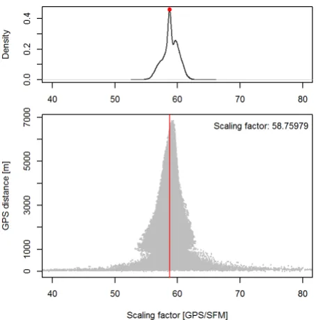
Figure 2 : Scale estimate between all possible point pairs. The figure showsthat points with short baselines should not be used to compute the scale (e.g. <500m). The relative length error coming from GPS location uncertainty is too large. Instead, when computing the density of scale distribution (upper panel) a consensus value is obtained.

Scale was obtained by computing the highest density of the probability density function of the ratio between pairs of points in model and cartographic coordinates (Figure 2 upper panel). Figure 2 (lower panel) shows that when points were less than 500m apart, the scatter of scale estimate was very large and converges for baselines longer than 1km. Such scatter comes from the imprecise GPS position determination.

Figure 3 : Rotation angle estimates with forward Monte-Carlo estimate. 20 thousand runs were computed in two passes. The first crudely determines the approximation value of omega, phi, kappa. A second pass of 20 thousand runs refines the domain where the optimal value lies. The optimal angle is then determined by robust least square fit of minimal RMSE on either side. These graphs for omega, phi, kappa, respectively cover the same angular span. Omega is the least well determined parameter as regression lines are flatter. On the other hand, for kappa, the solution is tighter. This comes from the acquisition geometry of the flight path. The overall RMS error where regression lines meet is 17.43m.

Inversion of rotation parameters is notoriously non-linear, which, with the presence of possible gross errors, may diverge. To circumvent this issue, we performed forward determination of Omega, Phi, Kappa angles with an intensive Monte-Carlo approach. In doing so, the rotation parameters are determined ISPRS Annals of the Photogrammetry, Remote Sensing and Spatial Information Sciences, Volume II-5, 2014

ISPRS Technical Commission V Symposium, 23 – 25 June 2014, Riva del Garda, Italy

(3)

without caring for non-linear behavior. The most likely value of each omega, phi, and kappa angle is that where minimum residuals converge (Figure 3). In Figure 3, it appears that Kappa (horizontal rotation about the vertical Z axis) is best determined because regression lines through minimum RMSE values are very steep. In the contrary, the Omega angle, translating a rotation about the horizontal X axis is not so well defined. This difference is behavior comes from the worse estimate of GPS elevation compared with X and Y. It should also be noted that the ranges of X and Y values are much broader (7 x 1 km) than that of Z values (only 0.2km).

Figure 4 : Translation estimates. Given the highly imprecise GPS coordinates, translations estimates are very variable. In order to reach some coherence, we picked the maximum of the kernel density estimation (with 2m bandwidth). Distributions are clearly non uni-modal and even though we picked the highest kernel density estimate, at least two values may work out for X and Y coordinates.

Translation parameter computation is also very sensitive to individual GPS errors (Figure 4). They were determined as the difference between scaled and rotated Model coordinates and cartographic GPS coordinates. Drawn as a histogram (Figure 4) in order to identify the most likely/frequent values, it appears that only the distributions of elevations are uni-modal with a single peak, even though it is not centered and symmetric. The translation in X is bi-modal, with a clearly higher peak, while the translation in Y is tri-modal, with two possible candidates.

The transformation from model coordinates to cartographic coordinates was than computed as the matrix product of five square 4x4 matrices so as to apply the final transform directly inside the Cloud Compare software.

Visual SFM coordinate convention is different from conventional right-hand direct axis scheme. This means that Y and Z coordinates need swapping (inside matrix M1) and inverting (inside matrix M2). Then a rotation matrix is applied (M3)which results from the multiplication of three individual rotation matrices Rkappa, Rphi and Romega, in this order, padding with the fourth line and column with zeros. Scaling (M4) is applied to the first three diagonal values. And finally, a translation (M5 with translations tx, ty and tz) finalizes the transform. “Mtot” provides the 4 x 4 matrix to paste into CloudCompare “Apply transformation” dialog box.

M1 = {1 0 0 0; 0 0 1 0 ; 0 1 0 0; 0 0 0 1}

M2 = {-1 0 0 0; 0 -1 0 0 0; 0 0 -1 0; 0 0 0 1}

M3 = {rot[1,1] rot[1,2] rot[1,3] 0; rot[2,1] rot[2,2] rot[2,3] 0; rot[3,1] rot[3,2] rot[3,3] 0; 0 0 0 1}

where rot = Rkappa * Rphi * Romega; using the sign convention scheme {cos x –sin x; sin x cos x}

M4 = {s 0 0 0; 0 s 0 0; 0 0 s 0; 0 0 0 1} (s = scale)

M5 = {0 0 0 tx; 0 0 0 ty; 0 0 0 tz; 0 0 0 1}

Mtot = M5 * M4 * M3 * M2 * M1

5. RESULTS

Using this solution scheme, SFM coordinates were transformed and compared to their respective GPS coordinates (Figure 5). For horizontal coordinates (Figure 5, left panel) the range of misfits reaches 100m. The vertical misfit range is smaller (Figure 5, middle and right panel). The distribution of errors is not uni-modal, as was already apparent during the determination of the model parameters. The cause of this could be an inhomogeneous behavior among cameras. As three simultaneous shots were acquired for each view points, we separated the misfits according to camera ID (NK1: left; NK2: middle and NK3: right camera). There does not seem to have a remarkable signature.

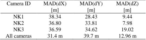
Statistically, the Median Absolute Deviation (MAD), which is the statistically robust equivalent of standard deviation for non-Gaussian distributions (Höhle & Höhle, 2009), contains 66% of the data and is compiled in Table 2. It appears that transformed SFM and GPS coordinates do not converge any better than within 30 meters horizontally and 12m vertically (Table 2). The reason why convergence is so poor remains undetermined.

Figure 5 : Comparison between transformed SFM view point coordinates and cartographic GPS coordinates according to camera ID. The misfit shows indeed a large range of errors (80 m in X; 120m in Y and 40m in Z). In map view, (left panel), all three cameras behaved coherently, even though two groups stand out.

Table 1: Median Absolute Deviation (MAD) of misfits between GPS and SFM transformed coordinates. The MAD robust criterion contains 66% of observations.

Camera ID MAD(dX) [m]

MAD(dY) [m]

MAD(dZ) [m]

NK1 38.34 28.43 9.44

NK2 36.80 33.81 7.98

NK3 36.59 34.62 19.02

All cameras 31.4 m 39.7 m 12.96 m

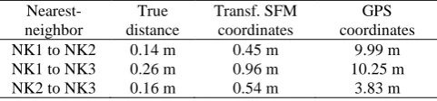
In this analysis we hypothesized that GPS coordinates are of poorer quality than SFM relative computation. This is demonstrated when comparing the distance between cameras at each trigger moments. To match synchronous triplets of photos, the distribution of the first SFM nearest neighbor distance was computed. Table 2 shows that the most frequent SFM inter-camera distance is three times larger than their true physical distance but the corresponding GPS distances are 10 to 20 times worse (Table 2).

ISPRS Annals of the Photogrammetry, Remote Sensing and Spatial Information Sciences, Volume II-5, 2014 ISPRS Technical Commission V Symposium, 23 – 25 June 2014, Riva del Garda, Italy

(4)

Table 2 : Most frequent nearest-neighbor distance between estimated camera viewpoints in transformed SFM coordinates and GPS coordinates.

Nearest-neighbor

True distance

Transf. SFM coordinates

GPS coordinates

NK1 to NK2 0.14 m 0.45 m 9.99 m

NK1 to NK3 0.26 m 0.96 m 10.25 m

NK2 to NK3 0.16 m 0.54 m 3.83 m

SFM point of views were computed based on SIFT points, whose existence is intrinsically controlled by image contents, and location controlled by camera geometry reconstruction. The cliff was roughly 600m away from the cameras. To scale, a pixel is ca. 8cm. This means that SFM viewpoint reconstruction is precise within 5 to 10 pixels; that is a relative precision scale of 1/600 to 1/1300. A better interior orientation that solves only three distinct cameras instead of 568 would improve matters. A further aspect is the crude default camera model used by Visual SFM, solving only one radial distortion parameter. A finer camera model would further tighten SFM view point reconstruction. Acting on these two aspects would improve the precision of view point reconstruction. Instantaneous GPS coordinates triplets show the intrinsic limitation of the Solmeta Geotagger Pro2 hardware. Such devices are very convenient and low-cost, but prove imprecise.

Does it matter? Most definitely. The cliffs and coastal platforms hence scaled and oriented show that sea level is tilted by about 2° along shore. Yet, no one in human history, even with the wildest effects of climate change, has ever noticed such tilt. Direct absolute orientation of SFM models can therefore not live with such imprecise GPS positions. Either differential GNSS tagging is required or Ground Control Points need be measured.

6. CONCLUSIONS

In this article, we examine the possibility to use Solmeta GPS geotagging units to orient structure-from-motion 3D point clouds of a coastal cliff without measuring Ground Control Points. The toy example was a set of 568 oblique stereo photographs acquired in a loop around a cliff of interest. A robust computation scheme was designed to retrieve the 7-parameters transforms between SFM and world coordinates to limit gross GPS location errors.

Misfits between GPS and SFM coordinates converge only to within several tens of meters. Default Visual SFM parameters achieved relative viewpoint precision comprised between 1/600 and 1/1300. Ways to improve these results is both by tightening the internal orientation parameter inversion - that is inverting only 3 cameras as opposed to 568 and refining the camera model – and by using differential GNSS aboard the plane and synchronizing the recorded track after the fact. Direct georeferencing with Solmeta Geotagger Pro2 proved inadequate to reconstruct a horizontal sea level.

7. REFERENCES

Ahmadabadian, A. H., Robson, S., Boehm, J., Shortis, L., Wenzel, K., Fritsch, D., 2013, Comparison of dense matching algoirthms for scaled surface reconstruction using stereo camera rigs, ISPRS J. of Photogramm., 78, 157-167.

Dewez, T., Rohmer, J., Closset, L., 2007. Laser survey and mechanical modeling of chalky sea cliff collapse in Normandy, France, in: McInnes, R., Jakeways, J., Fairbanks, H., Mathie, E.

(Eds.), Landslides and climate change, challenges and solutions, Taylor and Francis, London, pp. 281-288.

Dewez, T., Rohmer, J., Regard, V., and Cnudde, C., 2013. Probabilistic coastal cliff collapse hazard from repeated terrestrial laser surveys: case study from Mesnil Val (Normandy, northern France), J. Coast. Res., Sp. Iss. 65, 702-707.

Höhle, J. & Höhle, M., 2009, Accuracy assessment of digital elevation models by means of robust statistical methods, J. ISPRS, 64, 398-406.

James, M. R., and S. Robson, 2012, Straightforward reconstruction of 3D surfaces and topography with a camera: Accuracy and geoscience application, J. Geophys. Res., 117, F03017, doi:10.1029/2011JF002289.

Kraus, K., 1993, Photogrammetry volume 1: fundamentals and standard processes. Dummler Verlag, Bonn.

Lague, D., Brodu, N., Leroux, J., 2013, Comparison od complex topography with terrestrial laser scanner : Application to the Rangitikei canyon (N-Z), ISPRS J. of Photogramm., 82, 10-26.

Rosser, N.J., Petley, D.N., Lim, M., Dunning, S.A., Allison, R.J., 2005, Terrestrial laser scanning for monitoring the process of hard rock coastal cliff erosion, Quat. J., Eng. Geol. & Hydrogeol., 38, 363-375.

ISPRS Annals of the Photogrammetry, Remote Sensing and Spatial Information Sciences, Volume II-5, 2014 ISPRS Technical Commission V Symposium, 23 – 25 June 2014, Riva del Garda, Italy