ENHANCED COMPONENT DETECTION ALGORITHM
OF FULL-WAVEFORM LIDAR DATA
M . Zhou, M . H. Liu, Z. Zhang, J. H. Wang
Key Laboratory of Quantitative Remote Sensing Information Technology, Academy of Opto -Electronics, Chinese Academy of Sciences , Beijing, China – (zhoumei, liumenghua, zhangzheng, wangjinhu)@aoe.ac.cn
Commission VI, WG VI/4
KEY WORDS : Full-waveform LiDAR, Component detection, Waveform decomposition, LM , FM M
ABS TRACT:
When full-waveform LiDAR (FW-LiDAR) data are applied to extract the component feature information of interest targets, there exist a problem of components lost during the waveform decomposition procedure, which severely constrains the performance of subsequent targets information extraction. Focusing on the problem above, an enhance component detection algorithm, which combines Finite M ixed M ethod (FM M ), Levenberg-M arquardt (LM ) algorithm and Penalized M inimum M atching Distance (PM M D),is proposed in this paper. All of the algorithms for parameters initialization, waveform decomp osition and missing component detection have been improved, which greatly increase the precision of component detection, and guarantee the precision of waveform decomposition that could help the weak information extraction of interest targets. The effectiveness of this method is verified by the experimental results of simulation and measured data.
1. INTRODUCTION
Due to the fact that LiDAR can penetrate vegetation cover to get the elevation and the Earth topographic, it has the potential of extracting hidden targets. In this field, FW-LiDAR shows obvious advantages over traditional LiDAR, which just obtains elevation information from surface targets, since it can provide abundant features of vertical structure and surface, which reflect the inherent characteristics of the ground objects.
Factors such as the scattering characteristics of the target, the work mechanism of laser pulse, the difference of the number of component in a single pulse, contribute to the records of all the component waveform mixture making the valuable information difficult to obtain directly . Therefore, it is necessary to process the FW data, including the waveform modelling, pre-processing, waveform decomposition and component feature extraction. In the course of processing, waveform decomposition is the key step to get the accurate information of each component. For waveform decomposition, the Expectation M aximum (EM ) algorithm is more mature over the deconvolution (Wu, et al, 2011) and B-spline (Roncat, et al,2011). But the parameter initialization of the EM algorithm needs to pre-estimate the number of components and parameters of the component model (Wagner, et al,2006).
As to the parameters initialization of waveform decomposition, Persson et al. pre-estimate the number of components by using the Akaike Information Criterion (AIC). They use the generalized Gaussian function as the kernel function and
estimate the model parameters of backscattered echo waveform based on nonlinear least squares, then completed waveform decomposition initialization (Persson, et al, 2005). However, components will be missed when the waveform is complicated or the noise reduction is incomplete. Chauve et al. used a nonlinear least square curve fitting in combination with LM algorithm to detect waveform iteratively (Chauve, et al,2007). This method can detect missing components effectively, but it performs the curve fitting without waveform modelling and only takes the fitting residual minimum as the optimal conditions for the parameter initialization which will introduce an error and influence the effect of the component detection.
To solve these problems mentioned above, an enhance component detection algorithm is proposed in this paper, which combines FM M , LM algorithm and PM M D. All of the algorithms for parameter initialization, waveform decomposition and missing component detection have been improved, which greatly increase the precision of component detection.
2. METHOD
2.1 Finite Mixed Method (FMM)
In view of the fact that waveform decomposition based on the EM algorithm modelling the waveform by generalized Gaussian model shows as equation 1 (Chauve, et al,2007).
This paper takes the FM M to endow the weight for each component, which makes the modelled waveform more similar
2
the parameters associated with jth component. 1 2 1 2
( , , , , , , , )
k
k
Θ is the parameter vector which contains all parameters in the model (Geoffrey, et al, 2000).
2.2 Levenberg-Marquardt (LM)
LM algorithm is a Nonlinear Least Squares (NLS) fitting technique and uses self-iteration to determine whether there is a missing component. In contrast with the LM method after waveform decomposition, this paper utilizes the LM in the parameter initialization process to optimize the initialization of the components number. This method can enhance the efficiency of component detection and minimize the probability of missing components.
The fitting parameter
* is computed as follow:* * 2 allows us to estimate the number and the position of the echoes in order to initialize the NLS fitting. In the second step, additional peaks are searched in the difference between modelled and raw signals. If new peaks are found, the fit is performed again and its quality re-evaluated. The process is iterated until no further improvement is obtained. The selected solution is the model providing the minimum value for Eq. (5).
2.3 Penalized Minimum Matching Distance (PMMD)
PM M D method selects the number of mixture components that minimises the penalized matching distance between the PDFs estimated by the EM algorithm and Parzen’s method. It considers both of the conditions when the number of components is either too large (over-fitting) or too small (under-fitting). This method is leading into the process of component detection to judge whether there is a missing component after the first decomposition of the waveform in this paper. When the number of components is too large or too small, the PM M D will get significantly large. So the correct number of components in FM M can be determined by the choice of minimum distance value.
2.3.1 Estimation of PDF via Parzen’s method: Parzen provides a non-parametric method for estimating the PDF from a finite set of data (1) ( )
The matching distance
used in this paper is a measure for the similarity between two PDFsP
parzen( )
x
andPem( )x . It is2.3.2 Penalized matching distance: The motivation of our proposed penalized matching distance method is based on the following observation. When k is unnecessarily large, some of the mixing probabilities
{
j,
j
1,..., }
k
will be very small.As a result, their product
1 2... k will be also very small. Therefore, we are able to control the size of k by controlling the size of the
j’s. Hence, if we define the following penalty term:1 2 1 log
...
penalty
k
(9)
and add it to the matching distance
in Eq. (8), then we get the penalized matching distance as follows:penalty
(10)As we just discussed, for unnecessarily large k,
1 2... k willbe very small and
penaltywill be very large. So, large k is indirectly penalized if we choose the k* corresponding to theminimum penalized matching distance * as the number of mixture components. This is indeed quite important for the excellent performance of our algorithm, as it is shown in Section 3.
The operation carried out by the penalized minimum matching distance-guided EM algorithm is as follows. For each k(k=1,2,…), EM algorithm with the selected k is iterated until it converges to
. After that,
and
penaltyare calculated based on Eqs. (8) and (9). When it is over-fitted,
penaltywill be large; when it is under-fitted,
will be large. So the k*, which corresponds to the minimum*, is selected as the right number of mixture components. (Luo, et al, 2006)2.4 Algorithm Design
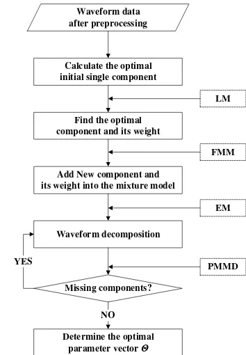
Through the analysis of the above methods, we summarized the algorithm as the following steps:
(1) As input is FW-LiDAR waveform data after filtering processing, use LM algorithm to estimate the probability density of sampling point intensity in a single pulse and calculate the optimal initial single component P1.
(2) Explore the best new component
f x
(
i|
*)
with its weight* i
in FM M model.(3) Add the detected component with its weight into the mixture model based on the principle of FM M model.
* *
1
( )
( )
( |
)
m m
P
x
P x
f x
(11)(4) Estimate and update parameters of each component using the EM algorithm until convergence.
(5) Calculate PM M D and determine the number of components. (6) Determine whether the iteration is terminated or not, and output the number of components and parameters of each component finally.
The flow char of the algorithm is shown in Figure 1.
Waveform data after preprocessing
Calculate the optimal initial single component
Find the optimal
componentand its weight
Waveform decomposition
EM
Missing components? YES
LM
NO
Determine the optimal
parameter vector Θ
Add New component and its weight into the mixture model
FMM
PMMD
Figure 1. Flow char of the component detection algorithm 3. EXPERIMENTAL RES ULTS
3.1 Experiment with S imulation Data
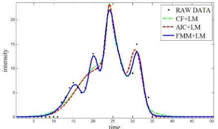
In this paper, we use simulation and measured data to validate the algorithm. As shown in Figure 2, the simulation data contains four components in a single back scattered pulse waveform. The sampling interval is 1ns and including 50 sampling points.
Figure 2. Simulated backscatter return waveform which contains 4 components
We compare our proposed algorithm with (1) curve fitting (CF) combined with the LM and (2) AIC combined with the LM .
The result is shown in Figure 3.
All waveform decomposition algorithms are based on EM algorithm, the only difference between these algorithms lie in the estimate of initial parameter in EM algorithms and the optimization of iterative decomposition results.
CF and LM oriented waveform decomposition algorithm (green - • -) and AIC and LM oriented (red ---) waveform decomposition can both discriminate the third and the forth components of the backward scattering waveform, but the first two components are missing; while FM M and LM oriented (blue -) waveform decomposition algorithm, which can identify all the four components of the scattering echo waveform, therefore greatly improve the component detection.
Figure 3. Waveform (simulated data) decomposition results based on three different methods
3.2 Experiment with Measured Data
The measured data are collected in September 2012 using the IGI's LiteM apper 5600 laser radar system at M iyun District of Beijing, and the point density is about 4 points/m2.
In order to prove the validity of the proposed algorithm, we select the measurement zone which may has multi components from the image of the measured area. We also compare our proposed algorithm with (1) CF combined with the LM and (2) AIC combined with the LM . The result is shown in Figure 4.
Figure 4. Waveform (measured data) decomposition results based on three different methods
All of the method can detect three components, but according to the detection results, FM M and LM algorithm can more accurately restore the components of the original waveform information, which are consistent with the original waveform data therefore is correct and validated.
Then we selected four types of data, including farmland, roads, forest land and buildings data, and use the data of the farmland as an example to show the detection results which contain 1, 2, 3 components data respectively . We use the raw data as ground truth and consider the variance and degrees of freedom of the hybrid model of waveform data after fitting to evaluate the effect of enhanced detection result (Chauve, et al, 2007):
2
1 1
[ ( )]
N
k k
k
y f x N p
(12)where N indicates waveform sampling number, p is the parameter number of waveform decomposition model.
The results of the AIC and LM combined algorithm is similar to the CF with LM . When the number of component is small, such as farmland, road and building, the AIC with LM and CF with LM algorithm are able to detect the components of the waveform completely and the is small. While the number of component is big, the AIC with LM and CF with LM algorithm wouldn’t detect completely and the
will be larger. The FM M with LM can detect the weak component in the waveform and in the is small in all the different types of the area.The proposed algorithm has 20% accuracy gain compared with the curve fitting and LM combined algorithm,
Method
CF+LM AIC+LM FMM+LM
Number
Number
Number
Number
1 411 1.0540 428 1.0366 407 0.8776
2 27 1.0280 10 0.7088 30 0.7018
3 0 —— 0 —— 1 0.6657
Total 438 1.0524 438 1.0291 438 0.8651
Table 1. The performance evaluation of waveform decomposition method ---- farmland
Type Number CF+LM
Factor
AIC+LM Factor
FM M +LM Factor
Road 337 0.9537 0.9167 0.8882
Forest 504 1.2040 1.445 0.9149
Building 434 1.0240 1.0460 0.8651
Table 2. The performance comparison of detection method
4. CONCLUS IONS
The component detection method we propose in this paper increase the accuracy of waveform decomposition by detecting all the components in the backward scattering echo waveform. The proposed method is applicable to the component detection of multi-component and complex waveform. There are obvious advantages for the multi-component detection such as hidden target and the weak component information. It can avoid loss of information of weak component, and provide effective support for subsequent data applications such as hidden target extracting, topographic mapping and digital city modelling.
5. ACKNOWLEDGEMENTS
The authors would like to thank the support from innovation project ―Research of Full-waveform LiDAR data processing and application technology oriented to fine classification‖ of Academy of Opto-Electronics, Chinese Academy of Sciences, No. Y12403A01Y.
REFERENCES
Chauve A., M allet C., Bretar F., Durrieu S., Deseilligny M ., Puech W., 2007. Processing full-waveform lidar data: M odelling raw signals. In: Proceedings of the ISPRS Workshop "Laser Scanning 2007 and SilviLaser 2007", Espoo, Finland, pp. 102-107.
Chauve A., Vega C., Durrieu S., Bretar F., Allouis T., Deseilligny M ., Puech W., 2009. Advanced full-waveform lidar data echo detection: Assessing quality of derived terrain and tree height models in an alpine coniferous forest. International Journal of Remote Sensing, 30(19), pp. 5211–5228
Geoffrey, M ., 2000. Adaptive Filtering and Change Detection. A Wiley-Interscience Publication, pp. 6-7.
Luo, W., 2006. Penalized minimum matching distance-guided EM algorithm. AEU - International Journal of Electronics and Communications, 60(3)
,
pp.235-239Persson, A., Soderman U., Topel J., Ahlberg S., 2005. Visualization and analysis of full-waveform airborne laser scanner data. In: ISPRS WG III/3, III/4, V/3 Workshop "Laser scanning 2005", Enschede, the Netherlands, pp. 103-108. Roncat A., Bergauer G., Pfeifer N., 2011. B-spline deconvolution for differential target cross-section determination in full-waveform laser scanning data. ISPRS Journal of Photogrammetry and Remote Sensing, 66(4), pp.418–428. Wagner, W., Ullrich A, Ducic V, M elzer T., Studnicka N., 2006. Gaussian decomposition and calibration of a novel small-footprint full-waveform digitizing airborne laser scanner. ISPRS Journal of Photogrammetry & Remote sensing, 60(2), pp.100-112.
Wu, J., Aardt J., Asner G., 2011. A comparison of signal deconvolution algorithms based on small-footprint lidar waveform simulation. IEEE Transactions on Geoscience and