THE EFFECTS OF AGGRESSIVE POLICING:
THE DAYTON TRAFFIC ENFORCEMENT
EXPERIMENT
Alexander Weiss
Indiana University, BloomingtonSally Freels
University of Illinois, ChicagoINTRODUCTION
Over the past several years, numerous essays have examined the deterrent effects of aggressive police patrol strategies like traffic law enforcement (Jacob and Rich, 1981; Sampson and Cohen, 1988; Wilson and Boland, 1978, 1981). This essay continues this line of research. It reports on the results of a field experiment in Dayton, Ohio, designed to measure the effects of traffic law enforcement on crime, arrests and traffic accidents.
The paper is organized as follows. First, we review some previous studies in this area. Next, we describe the design and analysis of the Dayton experiment. Finally, we discuss our findings and offer some suggestions for further research.
PREVIOUS RESEARCH
At the same time, other scholars suggested that some traditional police strategies might, indeed, be effective. Boydstun (1975), for example, found that “field interrogation”, the stopping and questioning of suspicious persons, was a deterrent to certain “suppressible” crimes. Another study suggested that the police could be more effective by carefully managing uncommitted patrol time (Tien, 1978). Sherman (1983) pointed out that, while the Kansas City experiment demonstrated that random patrol was largely ineffective, it was wrong to infer from those findings that all police patrol strategies were also ineffective.
Drawing on Wilson’s earlier work (1968), Wilson and Boland (1978) examined the relationship between policing “style” and deterrence. They suggested that police organizations and enforcement philosophies tended to differ by community and that communities with more “aggressive” or “legalistic” styles of law enforcement experienced lower levels of crime. Wilson and Boland argued that patrol strategies (at the extremes) could be classified as either “passive” or “aggressive”. In an aggressive department the officer “maximizes [his] interventions and observations of the community”. An officer in a passive department, by contrast, would “rarely stop motor vehicles to issue citations for moving violations…”.
As their measure of police aggressiveness, Wilson and Boland chose the number of traffic citations written per officer, suggesting that high levels of traffic law enforcement were consistent with professional and legalistic (aggressive) modes of policing.
Wilson and Boland argued that communities with a more aggressive patrol strategy (as measured by traffic law enforcement) would experience lower levels of crime (measured in this case by the incidence of robbery). They suggested that aggressiveness affects crime in two ways: indirectly and directly. By indirect effects they suggested that aggressive patrol reduces the robbery rate by changing the probability that an arrest will be made. That is, by stopping and questioning persons the police are more likely to detect contraband, interrupt plans for the commission of offenses and apprehend persons fleeing the scene of crimes. Direct effects, on the other hand, are those that occur through heightened police visibility. This means that the police can reduce crime by convincing offenders that they are more likely to be apprehended, a more traditional general deterrence perspective.
lower rates of robbery. Thus, they argued that, “citizens do not necessarily have to spend more money to get more law enforcement; they can get it by … maintaining a personnel, incentive and management system that delivers more law enforcement” (p. 378). Wilson and Boland suggested that some of the methodological problems in their study (e.g. simultaneity) could be controlled through, “carefully designed experiments that measure the effect of innovations in police strategies on crime rates”. They suggested further that, “[T]he next step would be to introduce a generally aggressive patrol strategy (street stops, high traffic citation rates, quick response time) in an experimental area of a city and compare the crime rate with that of a control area where the same number of officers follow a passive control strategy”.
Jacob and Rich (1981) challenged the Wilson and Boland findings. Specifically, they examined whether the effects of patrol aggressiveness previously discovered would also emerge in a study of several cities over time. Jacob and Rich examined the relationship between robbery rates and traffic law enforcement (as measured by traffic citation rates) in Atlanta, Boston, Houston, Minneapolis, Newark, Oakland, Philadelphia and San Jose for the period 1948 to 1978.
Their analysis found that the correlation between robbery rates and traffic citations in the same year, as well as those lagged by one year, varied considerably from city to city. In only two cities was the correlation strong and in the correct direction. Thus, they argued, “the number of moving violations is not a good indicator of police aggressiveness…”.
A replication of the Wilson and Boland study was conducted by Sampson and Cohen (1988). They analyzed data from 171 American cities with populations of over 100,000 (a much larger sample than either previous study). Their definition of patrol aggressiveness suggested that officers in aggressive organizations would “stop motor vehicles to issue traffic citations at a high rate…”. Specifically, they used the number of arrests per officer for driving under the influence and for disorderly conduct as their measure of police aggressiveness.
effects of proactive policing, [should include] experiments whereby police strategies are randomly assigned to different areas”.
RESEARCH QUESTIONS AND HYPOTHESES
This study seeks to resolve several issues arising from previous research on the relationship between aggressive police patrol and crime. First, we agree that an experimental test of this question would be valu-able, particularly given the problems of simultaneity and measurement error present in other research. While previous studies have used sophis-ticated statistical techniques to control for the “natural” variation between the communities, such controls are often problematic. As Zimring (1976) has argued, “I do not believe that our present knowledge…permits us to control statistically for all the differences between South Dakota and New Jersey…”.
Next, we believe that aggressive policing needs to be more precise-ly operationalized. Consider, for example, the use of traffic citations as an indicator of policing style. If general deterrence is enhanced through police visibility, then simply counting the number of citations written (rather than the number of vehicles stopped) might significantly underestimate the true amount of “dosage”. For example, using citation rates might not allow a researcher to distinguish between styles of policing in two departments when the organizations stop about the same number of vehicles, but officers in one department write more tickets than officers in another.
Sampson and Cohen’s use of arrests for driving under the influence (DUI) as an indicator of aggressiveness is particularly troublesome because the DUI arrest decision is influenced by a number of factors other than policing style (Mastrofski, Ritti and Snipes, 1994; Weiss, 1992).
Our study will test four hypotheses:
H1: that areas subjected to increased levels of traffic law enforcement will experience lower levels of suppressible street crime;
H2: that increased traffic law enforcement will result in increased arrests for serious offenses;
H3: that increased traffic law enforcement will result in increased arrests for drugs, weapons and DUI;
METHODS
Research Design
In this evaluation we employed an interrupted time series design with a non-equivalent, no-treatment control group time series (Cook and Campbell, 1979). These designs are quite common in studies of general and specific deterrence (Campbell and Ross, 1971; Ross, 1967; Ross, McCleary and Epperlein, 1982). In the notation of Campbell and Stanley (1963) this design can be diagrammed as follows:
O1O2O3O4OnX1 O1O2O3O4On —————————
O1O2O3O4On O1O2O3O4On
where each O represents an observation and an X represents the introduction of a treatment. In this design, a control group is chosen on the basis of its comparability with the treatment group. The researcher seeks to match the two areas on as many dimensions as possible, particularly those which appear to be relevant to the research questions.
Interrupted time series designs are particularly effective in controlling for four threats to validity: history, maturation, instrumentation and other cyclical patterns (Cook and Campbell, 1979).
The addition of the nonequivalent control group adds significantly to our ability to control for history. For example, let us say that our outcome had been influenced by some factor like the weather. We would expect that such an influence would have had similar effects on both the experimental and control conditions.
Site Selection
Researchers placed announcements about the project in several police publications in order to identify potential sites. In consultation with the experiment’s sponsor, researchers narrowed the list of eligible agencies to five. In anticipation of final site selection, research staff visited several candidate sites to assess the availability of data. Finally, two sites were identified: Dayton, Ohio and Baltimore County, Maryland1.
The Dayton Traffic Enforcement Experiment
The Dayton Police Department was a particularly attractive site for this research. It was relatively large (457 sworn officers), but not so large so that generalizability would be an issue. Second, the department had no specialized traffic division. That was important because whatever traffic enforcement was done would be done as part of a patrol officer’s routine assignment; that is, it would be more characteristic of an overall policing “style”. Finally, the department was very enthusiastic about participating in the experiment.
After Dayton was chosen, it was necessary to identify the areas within the city that would be used for the experiment. We asked the police department to identify six to eight potential sites. We asked that the sites had certain characteristics. First, we looked for areas that included a high volume arterial street with a mix of commercial property and high and low density residential property. Second, we sought areas that had been relatively stable over time. Third, we wanted areas that had experienced substantial levels of crime and traffic accidents. Finally, we asked that the sites not be contiguous.
After the agency identified potential sites, one area was randomly chosen to be the experimental (treatment) area and another was selected to be the control (comparison) area.
Implementation
Prior to the start of the experiment, researchers visited the site to meet the participating police officers. Officers assigned to evening and night shifts were briefed on the project and given a document that described the objectives of the project. Several briefings were given because of the shift rotation. Some officers probably did not receive the initial briefing but did receive the briefing documents.
Of particular concern was the integrity of the treatment regimens. We believed that increasing the number of traffic stops in the experimental areas would increase visibility in two ways. First, motorists and pedestrians in the experimental area would have a heightened awareness of police presence. Interestingly, the topography of the site was such that a vehicle stopped by the police could be observed at any point along the road segment. Second, we expected that those who observed the increased police presence would tell others.
Given these objectives, officers were told to enforce traffic laws aggressively in the experimental areas, with particular emphasis on the period of 6.00 p.m. to midnight. While they were encouraged to write citations, they were told that vehicle stops were equally critical. We encouraged officers to handle these traffic contacts as they would have under normal circumstances. Officers were told to make the stops in locations easily visible to other motorists and to activate their emergency lights. There were no briefings or special instructions given to officers in the control areas, but their commanding officers were informed about the project. Because we were interested in testing the independent effects of police activity, there was no publicity about the project or about the activities of the officers involved. The experiment began in Dayton on January 6 1992. It lasted for six months.
Site Management and Coordination
Conducting experiments in field settings is often difficult and this one was no exception (Riecken and Boruch, 1974). However, because of a high degree of interest in the experiment by department administrators (a lieutenant from the chief’s staff was assigned as project liaison) and particularly strong support from field commanders (the district commander was very interested in the experiment), the problems were relatively minor. Researchers made periodic site visits. On those occasions we met with department representatives, briefed officers involved in the project and observed police activity in the experimental area, both by covertly observing the experimental area and by riding with officers participating in the experiment.
Data Collection
Four kinds of data were collected:
(1) treatment levels,
(2) crime incidence,
(3) arrests, and
(4) traffic accidents.
Data were collected for the police reporting areas that either included or were adjacent to the treatment and control areas. While the experiment was conducted primarily during the hours of 6.00 p.m. to midnight, data were collected for the entire 24-hour period. Data for the outcome measures were collected for the three years prior to the beginning of the experiment and for the six-month experiment. Data for the traffic stops in Dayton were only collected for the duration of the experiment, because it was not available for the pre-experimental period2.
Treatment Measures
Crime Incidence
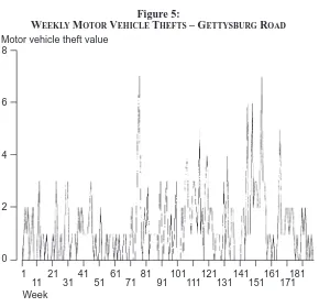
We employed two alternative measures of crime incidence. The first (drawing on previous research) was the number of robberies3. The second was the incidence of auto theft. We believed that this offense was well suited to our study of deterrence because auto theft generally takes place in areas subject to police observation.
Arrest Data
Two types of arrest data were collected. First, we collected data for all index arrests, including arrests for auto theft and robbery. Second, we collected data on “special” arrests, involving weapons, drugs (both sales and possession) and DUI. We should note that some of the arrests recorded were for offenses that may have occurred outside of the treatment and control areas. Moreover, some of the arrests may have been made by officers not participating in the experiment4.
Accident Data
Finally, we gathered data for all reported traffic accidents. In general, these included accidents in which a person was either injured or killed, or in which a tow truck was required to clear the accident scene5.
Data Analysis
Techniques for the statistical analysis of time-series quasi-experiments are based on the autoregressive integrated moving average (ARIMA) models of Box and Jenkins (1976) and Box and Tiao (1975). The analysis consists of an iterative process of model identification, estimation and diagnosis. These techniques are described in detail in McCain and McCleary (1979), McCleary, Hay and Meidinger (1980) and McDowall, McCleary and Meidinger (1980).
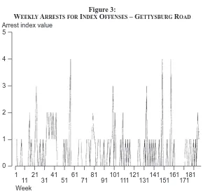
Our analysis of data for the Dayton experiment will consist of three parts. First, we examine the graphical presentations of the outcome measures. Second, we attempt to identify the ARIMA model. Finally, we provide estimates of program effects.
and then for Keowee Street (control). Tables 1 and 2 illustrate the summary measures for these outcome measures. In addition, these tables include a measure of treatment delivery. As can be seen, officers in the experimental area made three times the number of stops as those in the control area.
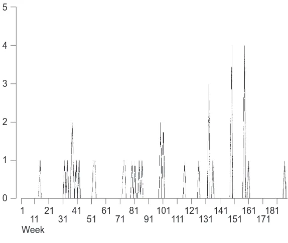
Figures 1 through 6 illustrate the weekly observations for our six outcome measures on Gettysburg Road. In Dayton, the experiment began on January 6 1992 (at week 158). The only effect demonstrated in these plots is the apparent reduction in “special” arrests.
After our initial observation of the time-series data, we then proceed to the ARIMA model identification. The basic approach to identifying an ARIMA model is to examine the plots of the autocorrelation functions (ACF) and partial autocorrelation functions (PACF). These analyses were conducted with the ARIMA procedure in SAS, a popular program for Box-Jenkins-type models.
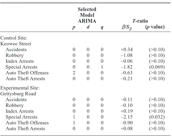
Table 3 illustrates the results of the model identification process. For each outcome measure, we observe the selected model based on the SAS analysis. For each model, we include the parameter estimates for autoregression ( p), stationarity (d ) and moving average (q). After identifying the appropriate noise model, we then turn to the test of the effect of the intervention. This is done by entering a term in the model that is coded for all pre-intervention observations and “1” for all post-intervention observations. We can then test for the significance of this coefficient to measure the effect of the treatment.
Returning to Table 3, we see the results of this analysis. For the models, we report the T-ratio and its associated probability value. The T-ratio is calculated by dividing the estimated coefficient by its
Table 1
SUMMARYMEASURES(MEANS) FORWEEKLYDATA: GETTYSBURGROAD
Measure Pre-Test Post-Test
Accidents 4.1 4.1
Robbery 1.12 1.1
Index Arrests 0.53 0.56
Special Arrests 2.9 1.8
Auto Theft Offenses 1.3 1.03
Auto Theft Arrests 0.19 0.2
standard error. The sign before each T-ratio indicates the direction of the effect. For coefficients to be statistically significant at the 0.05
12
WEEKLYTRAFFICACCIDENTS– GETTYSBURGROAD
Table 2
Auto Theft Offenses 2.1 1.9
Auto Theft Arrests 0.2 0.2
confidence level, T-ratios must generally exceed 2 and probability values must be less than 0.05.
As we can see, the only outcome measure that is statistically significant is special arrests for Gettysburg Road. However, the sign of the coefficient is in the opposite direction of what we had hypothesized.
DISCUSSION
Previous research has suggested that a relationship exists between aggressive policing (as measured by the level of traffic enforcement) and crime. It has been suggested that the effect of traffic enforcement can be either “indirect” (i.e. that traffic enforcement will
5
4
3
2
1
0
Robbery value
Week 1
11 21 3141 51 6171 81 91101111121131141151161171181
Figure 2:
result in the detection of fugitives and contraband) or “direct” (by changing perceptions of the likelihood of arrest). Two studies (Sampson and Cohen, 1988; Wilson and Boland, 1978) concluded that communities that experienced higher levels of traffic law enforcement also experienced lower rates of robbery.
We were unable to replicate either the Wilson and Boland or Sampson and Cohen findings. First, we found no evidence that increased traffic enforcement reduces the incidence of either robbery or auto theft, nor does it effect arrests for index offenses. We failed to detect any effect on reported traffic accidents.
Our findings with respect to indirect effects are more problematic. We had hypothesized that increasing vehicle stops would result in increased arrests for drugs, weapons and DUI. In fact, the result was a statistically significant reduction in these arrests.
5
However, a similar result (although not statistically significant) occurred in the control area, suggesting the influence of some extraneous factor.
There are three reasons why this study may have failed to detect a relationship between traffic enforcement and crime: the absence of such a relationship, an insufficient level of treatment and inadequate statistical power.
First, it may be that the reason why our study failed to detect a relationship between traffic enforcement and crime is because none exists. This finding would be consistent with Jacob and Rich (1981) who concluded that there was a weak relationship between levels of traffic enforcement and crime over time in several cities. Recall that while previous studies used traffic enforcement as a surrogate measure of patrol aggressiveness, our study tested its direct effect. It may be that traffic enforcement and aggressive policing are not the same thing. While traffic
14
12
10
8
6
4
2
0
Specimen arrest value
Week 1
11 21 3141 51 6171 81 91101111121131141151161171181
Figure 4:
enforcement may be effective as part of an aggressive policing strategy, it may be less effective when it is the entire strategy.
It is important to point out that we did not set out to measure the effects of traffic contacts on particular individuals or with regard to specific offenses. Had we done so, the results might have been different. In a recent study, for example, researchers in Kansas City (Sherman, Shaw and Rogan, 1995) found that police patrols in “hot spots” of crime and targeted towards “high risk” offenders, resulted in an increase in gun seizures and a reduction in gun crime.
Second, our findings may have resulted because the level of traffic enforcement delivered was insufficient. Even though there was confor-mance with the experimental protocol (officers in the experimental area stopped three times as many vehicles as those in the control), the level of traffic stops was still rather modest (34 per week). It may be that there is a relationship between traffic enforcement and crime but that it requires a substantial level of effort greater than was available in this experiment.
While there is anecdotal evidence that “routine” traffic stops result in the arrest of serious offenders (Karr, 1995), it is unclear whether increasing the frequency of traffic stops will result in a proportional increase in arrests.
Finally, the experimental results may have occurred because our study lacked sufficient statistical power; that is, the magnitude of the effect was not sufficiently large to be able to rule out chance occurrences. This is a common problem in field experiments. Although they were of insufficient magnitude, some of the parameter estimates were in the hypothesized direction. A finding of nonsignificance does not necessarily show the absence of an effect, but rather the inability of the model to detect such an effect. For example, there was a 5.2 percent increase in arrests for auto theft in the experimental area. Although we could not rule out such a result having occurred by chance, this is clearly an increase in productivity that is of interest to policymakers. Unfortunately, techniques for conducting
5
4
3
2
1
0
Motor vehicle theft arrest value
Week 1
11 21 3141 51 6171 81 91101111121131141151161171181
Figure 6:
power analyses in interrupted time-series experiments are not sufficiently developed to be of use in this case (Judd and Kenney, 1981).
CONCLUSION
Like many field experiments, the Dayton Traffic Enforcement Experiment suggests some opportunities for further research. Clearly, our ability to examine these questions would be enhanced through a randomized field trial with multiple treatment and control areas and multiple treatments, including enhanced enforcement, removed enforcement and designs that include the introduction and removal of treatments. Recent experience suggests that experiments of this type would be difficult but feasible (Sherman, 1992).
Given public concern about high levels of violent crime, police managers are seeking alternative allocation strategies. One such strategy might include increasing the level of traffic enforcement. This study
Table 3
TESTS FOR THEEFFECT OF THEINTERVENTION INDAYTON Selected
Model
ARIMA T-ratio
p d q β/Sβ (p value)
Control Site: Keowee Street
Accidents 0 0 0 +0.34 (>0.10)
Robbery 0 0 0 –1.08 (>0.10)
Index Arrests 0 0 0 –0.06 (>0.10)
Special Arrests 0 0 1 –1.82 (0.069)
Auto Theft Offenses 2 0 0 –0.63 (>0.10) Auto Theft Arrests 0 0 0 –0.21 (>0.10)
Experimental Site: Gettysburg Road
Accidents 0 0 0 –0.11 (>0.10)
Robbery 0 0 0 –0.10 (>0.10)
Index Arrests 0 0 0 +0.19 (>0.10)
Special Arrests 1 0 0 –2.15 (0.032)
provides no clear evidence that providing more traffic law enforcement will reduce crime. For now the relationship between aggressive policing and crime remains uncertain.
NOTES
1. This experiment was conducted in both sites; however, several events at the Baltimore site resulted in an unsuccessful implementation of the treatment. In fact, the amount of traffic enforcement in the experimental area was lower than before the project. While the Baltimore results are not reported here, a complete description is available in the final report to the National Highway Traffic Safety Administration
2. We used a daily activity report to measure traffic stops during the experiment. We attempted to estimate the level of pre-intervention traffic contacts using CAD data. However, because many officers fail to notify dispatchers when making traffic stops, this method was largely unsuccessful
3. Our use of robbery as an outcome measure is problematic because it includes all categories of robbery. We employed this measure because it was the same used by Wilson and Boland and by Sampson and Cohen. Thus, it was the only measure comparable across studies.
4. Using arrests as a measure of impact can be troublesome because the number of arrests is in large part a measure of productivity. However, previous studies have suggested that increasing vehicle stops will likely lead to more contact with vehicles containing contraband. If this is true, more arrests should result. It is clear, however, that the number of arrests in this experiment was not a measure of treatment, but one of impact.
5. While this measure is only marginally related to the question under study, its inclusion was mandated by the project’s sponsor.
REFERENCES
Box, G.E.P. and Jenkins, G.M. (1976), Time Series Analysis: Forecasting and
Control, Holden-Day, San Francisco, CA.
Box, G.E.P. and Tiao, G.C. (1975), “Intervention analysis with applications to economic and environmental problems”, Journal of the American Statistical
Boydstun, J. (1975), San Diego Field Interrogation: Final Report, Police Foundation, Washington, DC.
Campbell, D.T. and Ross, H.L. (1971), “The Connecticut crackdown on speeding: time series data in quasi-experimental analysis”, Law and Society Review, 3:33-53.
Campbell, D.T. and Stanley, J. (1963), Experimental and Quasi-experimental
Designs for Research, Rand-McNally, Chicago, IL.
Cook, T.D. and Campbell, D.T. (1979), Quasiexperimentation: Design and
Analysis Issues for Field Settings, Rand-McNally, Chicago, IL.
Greenwood, P., Chaiken, J. and Petersilia, J. (1977), The Criminal Investigation
Process, D.C. Heath, Lexington, MA.
Jacob, H. and Rich, M.J. (1981), “The effects of police on crime: a second look”,
Law and Society Review, 15:109-15.
Judd, C. and Kenny, D. (1981), Estimating the Effects of Social Interventions, Cambridge University Press.
Kansas City Police Department (1977), Response Time Analysis: Executive
Summary.
Karr, A.R. (1995), “Police capitalize on common failing of criminals: they break the law”, Wall Street Journal, May 18:B1.
Kelling, G.L., Pate, T., Dickman, P. and Brown, C. (1974), The Kansas City
Pre-ventive Patrol Experiment: Technical Report, Police Foundation, Washington, DC.
McCain, L.J. and McCleary, R. (1979), “The statistical analysis of the simple interrupted time-series quasi-experiment”, in Cook, T.D. and Campbell, D.T.,
Quasiexperimentation: Design and Analysis Issues for Field Settings,
Rand-McNally, Chicago, IL.
McCleary, R., Hay, R.A., Meidinger, E.E. and McDowall, D. (1980), Applied
Time Series Analysis for the Social Sciences, Sage, Beverly Hills, CA.
McDowall, D., McCleary, R., Meidinger, E.E. and Hay, R.A. Jr (1980),
Interrupted Time Series Analysis, Sage, Beverly Hills, CA.
Mastrofski, S.R., Ritti, R.R. and Snipes, J. (1994), “Organization theory and police arrests: expectancy theory and police productivity in DUI enforcement”,
Law and Society Review, 28:113-48.
Riecken, H.W. and Boruch, R.F. (1974), Social Experimentation: A Method for
Ross, H.L. (1967), “Law, science, and accidents: the British Road Safety Act of 1967”, Journal of Legal Studies, 2:1-78.
Ross, H.L, McCleary, R. and Epperlein, T. (1982), “Deterrence of drinking and driving in France: an evaluation of the Law of July 12, 1978”, Law and Society
Review, 16:345-74.
Sampson, R.J. and Cohen, J. (1988), “Deterrent effects of the police on crime: replication and theoretical extension”, Law and Society Review, 22:163-89.
Sherman, L.W. (1983), “Patrol strategies for the police”, in Wilson, J.Q. (Ed.),
Crime and Public Policy, ICS Press, San Francisco, CA.
Sherman, L.W. (1992), Policing Domestic Violence, Free Press, New York, NY.
Sherman, L.W., Shaw, J. and Rogan, D. (1995), The Kansas City Gun
Experiment, National Institute of Justice, Washington, DC.
Tien, J.M., Simon, J.W. and Larson, R. (1978), An Alternative Approach to Police
Patrol: The Wilmington Split-Force Experiment, Law Enforcement Assistance
Administration, Washington, DC.
Weiss, A. (1992), “Determinants of police DWI policy making”, Alcohol, Drugs,
and Driving, 7:221-8.
Wilson, J.Q. (1968), Varieties of Police Behavior, Harvard University Press, Cambridge, MA.
Wilson, J.Q. and Boland, B. (1978), “The effect of the police on crime”, Law and
Society Review, 12:367-90.
Wilson, J.Q. and Boland, B. (1981), “The effects of the police on crime: a rejoinder”, Law and Society Review, 16:163-9.