TOWARDS TRANSPARENT QUALITY MEASURES IN SURFACE BASED
REGISTRATION PROCESSES: EFFECTS OF DEFORMATION ONTO COMMERCIAL
AND SCIENTIFIC IMPLEMENTATIONS
D. Wujanz
Berlin Institute of Technology
Department of Geodesy and Geoinformation Science Chair of Geodesy and Adjustment Theory Strasse des 17. Juni, 10623 Berlin, Germany
[email protected] www.geodesy.tu-berlin.de
Commission V, WG V/3
KEY WORDS: TLS, Registration, Point Cloud, Accuracy, Quality, Deformation
ABSTRACT:
Terrestrial Laser Scanners have been widely accepted as a surveying instrument in research as well as in commercial applications. While aspects of scanner accuracy and other influential impacts onto the measured values have been extensively analysed, the impact of registration methods and especially the assessment of transformation parameters remained outside the scientific focus. To this day the outcome of a surface based registration, such as ICP or 4PCS, is usually described by a single number representing several thousand points that have been used to derive the transformation parameters. This description neglects established perceptions in geodesy where for instance distribution, size of all derived residuals and its location are considered. This contribution proposes a more objective view on the outcome of registration processes and compares new approaches to results derived with commercial solutions. The impact of deformation is also analysed in order to determine if available solutions are able to cope with this problem.
1. INTRODUCTION
Due to the fact that Terrestrial Laser Scanners (TLS) are only capable of capturing visible areas of an object from one standpoint further perspectives are needed in order to fully describe a surveyed object within a local 3D Cartesian coordinate system whose origin is located in the centre of the instrument. Thus the necessity arises to survey the object from several standpoints and assemble these captured fragments to a complete model. This spatial rigid body transformation, also referred to as registration or matching, is described by six parameters consisting of three translations tx, ty and tz and three rotations rx, ry and rz while the scale factor m stays uniform.
Several methods have been developed to identify corresponding points between datasets which satisfies the need of common information in two coordinate systems namely start system S and target system T. These correspondences are then used to integrate S into T by estimating suitable transformation parameters within an over-determined transformation. This can be achieved by providing surveyed targets in a local or superior coordinate system while all other methods rely on overlap between adjacent point clouds from which tie points can be extracted in various ways that can be categorised as follows:
Use of radiometric information such as intensity values (e.g. Böhm & Becker, 2007),
utilisation of geometric primitives for instance planes or cylinders (e.g. Gielsdorf et al., 2008),
surface based methods: e.g. Besl & McKay’s algorithm (1992), CHEN & Medioni’s contribution (1991) or Bae & Lichti’s (2008) approach.
Impacts onto the result of such a transformation are caused by the choice of the matching algorithm itself (Dold et al., 2007) as well as its implementation (Rusinkiewicz & Levoy, 2001). Further falsification is provoked by the geometric quality of all used points which has been analysed by Boehler et al. (2003) or the setup of the scanner in relation to the object (Soudarissanane, 2011).
1.1 Motivation
The motivation for this contribution can easily be justified by the lack of fully automated algorithms for transformation of two or more point clouds without adding physical targets to a scene. Demands of quality assurance fortify this aspect as quality measures are needed in order to verify automatically derived transformation parameters. Based on the lack of meaningful quality measures novel approaches are presented in this contribution. Furthermore erroneous or falsified results have to be detected which for instance can be caused by deformation. It should be mentioned that deformation occurs in nearly every scan due to the sequential and time consuming data acquisition process of TLS. Objects that very likely cause such geometric changes between two scans are for instance cars, pedestrians, trees or cranes at construction sites.
1.2 Peculiarities of Deformation Processes
In general two forms of appearance can be categorised for deformation processes: non-rigid body deformation and rigid body motion. The first type can be expressed by an alteration of shape, e.g. dilatation or torsion, translation and orientation of an object. These influences increase the amount of deviators within International Archives of the Photogrammetry, Remote Sensing and Spatial Information Sciences, Volume XXXIX-B5, 2012
a computation of transformation parameters and thus lead to falsification in case that these points are not withdrawn from the computation. Deformations of this type occur very likely in nature for instance on glaciers, melting of snow and ice, lava flows or sand dunes. The second form, where only location and alignment of objects vary, can lead to even larger problems. Depending on the quota of altered content one could misleadingly draw the conclusion that static objects appeared to have moved. This effect can be observed for instance in scenes that contain vehicles or cranes.
1.3 Description of a Perfect Matching Algorithm
Many approaches for the transformation of 3D datasets have been proposed but up till now no universally applicable method has been developed. The following list contains already existing requirements onto matching algorithms and adds much needed capabilities that would define a perfect solution:
Usable on datasets that contain regular and irregular shaped objects e.g. urban respectively natural scenes Possibility of integrating several information sources:
e.g. usage of geometric primitives, radiometric and surface based information
Robust against noise, outliers, deformations
Algorithm always computes the same results on same datasets (no random influences)
Common adjustment of multiple datasets Transparent and reliable quality assurance
Usage of adjustment calculation in order to determine accuracy and reliability of the computed parameters Control on adjustment / introduction of weights Introduction of conditions within an adjustment in
order to fix single parameters for instance that the alignment of the Z-axis has to remain the same.
The contribution at hand is structured in three major paragraphs where section 2 gives an introduction into the applied surface based matching algorithms while section 3 compares the behaviour of implementations namely Leica Cyclone, Raindrop Geomagic, GFaI Final Surface and the 4-points congruent sets algorithm, against deformations. Section 4 proposes novel quality measures in order to evaluate the outcome of the matching process and input data itself.
2. SURFACE BASED MATCHING ALGORITHMS
The following sections provide a brief introduction to basic surface based algorithms as they are up till now the most widespread category of surface matching approaches compared to the other two previously mentioned categories. Their robustness against deformations are analysed subsequently in section 3.
2.1 Iterative Closest Point Algorithm
The iterative closest point algorithm (ICP), presented in 1992 by Besl & McKay, is commonly used for registration processes and is implemented in most 3D processing software packages. The ICP relies on a coarse alignment of two overlapping datasets in order to avoid falling into a local minimum of the target function. A set of randomly sampled closest point pairs is minimised in terms of applying a mean-square distance metric. During each iterative step transformation parameters are
computed that are evaluated by the previously mentioned error metric. The algorithm terminates when the outcome of the error metric has fallen below a preset threshold. Some implementations use a maximum search distance during nearest neighbour determination in order to avoid influences caused by outliers.
2.2 4-Points Congruent Sets Registration
A weak spot of the above mentioned ICP algorithm is its dependence to a coarse alignment which still requires user interaction. Aiger et al. (2008) introduced a solution to this problem with their 4-points congruent sets algorithm (4PCS) which does not need any approximate values concerning the starting alignment of two overlapping datasets. The authors claim that this high-performance solution is resilient against noise and outliers even without previously performed blunder detection or filtering. The approach can be applied to point clouds and meshed surfaces applying a rigid transformation to one of the datasets. The basic idea behind this algorithm is to extract sets of four points that are coplanar to a certain degree and to find their corresponding partner by means of approximate congruency. Several control parameters of the 4PCS can be set while delta describes the degree of uncertainty concerning the average distance between points from two datasets and is measured by a fraction of the arithmetic mean. The estimated overlap is the main reason for the claimed stability of 4PCS as this characteristic is responsible for the composition and size of four point sets. The parameter n, which describes the applied number of randomly chosen points, is used to verify the computed transformation parameters and thus describes a control sample. A threshold t is used to evaluate the current set of transformation parameters and is also introduced as a stopping criterion. Furthermore t is the only implemented quality measure of the approach and is described by a ratio between the points that satisfy delta and are hence usually a fraction of n. Finally information on the deviation of surface normal can be introduced in order to filter the selected amount of points.
3. PRACTICAL COMPARISON OF SURFACE BASED MATCHING ALGORITHMS
In this section different algorithms and commercial products have been compared concerning their capabilities in terms of their implemented quality assurance measures as well as their behaviour against deformed areas. Therefore two datasets have been used:
1. Two point clouds with a partial overlap which do not contain any deformed areas (ISPRS reference dataset of the Golden Buddha statue located in Bangkok, Thailand); referred to as “buddha” in the following 2. Two point clouds with nearly complete overlap
featuring non-rigid body deformation which is subsequently denoted as “snow”.
3.1 Analysis of point clouds without deformation
In order to identify potential differences in implementation and characteristic behaviour of all algorithms the “buddha” datasets have been registered by applying all tested solutions with default settings. The scene contains a statue of a golden Buddha in lotus pose which measures approximately 8 m in width, is roughly 4 m long and about 10 m in height. The average International Archives of the Photogrammetry, Remote Sensing and Spatial Information Sciences, Volume XXXIX-B5, 2012
matching error, which describes the average spatial distance between corresponding points, derived with Geomagic was 62.2 mm based on 5000 points while Final Surface computed an error of 26.9 mm from 4499 points. Cyclone calculated an average deviation of 15.1 mm based on 8333 points while the 4PCS led to an error of 30.2 mm and a score of 80.1 %. This simple analysis reveals two curious characteristics which are the large spectrum of the quality measures on one hand as well as the significant differences of the individual transformation parameters on the other as outlined in Table 1. Due to the fact that no reference values for this dataset are given, no detailed information on the implemented error metric and corresponding point distribution on the object’s surface are given one can only speculate which solution delivered the best result.
Table 1: Comparison of all obtained transformation parameters Result tx [m] ty [m] tz [m] rx [°] ry [°] rz [°] Geomagic 0.041 13.208 -0.109 -0.146 -0.059 179.784 Final Surf 0.128 12.780 -0.409 0.645 1.496 176.965 Cyclone 0.043 13.187 -0.129 0.120 0.023 179.688 4PCS -0.205 12.920 0.004 1.088 3.742 179.422
3.2 Analysis of point clouds with deformation
The “snow” dataset features two epochs of a roof section, see
Figure 3. A snow mantle of roughly 16 cm can be found on the roof in the first dataset while most of the snow has melted when the second point cloud has been captured. In order to provide a reference set of transformation parameters all “deformed” areas that are covered by snow have been removed before the registration process has been started in Final Surface. The matching error of the reference set added up to 3.9 mm based on 2509 points which represented the best 50% of the matching points. Table 2 shows the reference values for the second dataset below. The major aim of this experiment is to determine the stability of all algorithms against datasets that contain outliers in form of deformation. Hence the “snow” scene has been processed including the snow cover to provoke potential effects. Furthermore the impact of tunable parameters onto the final result respectively their quality measures should be determined if possible.
Table 2: Reference transformation parameters tx [m] ty [m] tz [m] rx [°] ry [°] rz [°] -0.007 0.046 0.125 0.203 -0.145 10.633
3.2.1 Raindrop Geomagic Studio 12: Raindrop’s Geomagic Studio is able to perform transformations by using geometric primitives and a surface based matching algorithm. The only implemented quality measure is the average distance between two datasets while a colour coded inspection map can be computed if one of the point clouds has been converted into a meshed surface representation.
Figure 1: Colour coded visualisation of deformations: Based on reference transformation parameters and Result 2 derived by
Geomagic (right)
The outcome of the surface based matching can be influenced by the sample size and a maximum tolerance setting. It is worth mentioning that no initial alignment of the datasets is needed which works in most cases. Figure 1 shows a colour coded visualisation of computed deformations. It can notably be seen that the dataset on the left side, which has been computed by applying the reference parameters, shows only deformations on the roof (blue shades) caused by the snow as expected. The yellow patterns in the windows are effected by blinds that have been lowered in between epochs. A look on the right half of the image would lead to the conclusion that the wall as well as the roof would lean forward as indicated by the colour coding. Table 3 gathers all produced results where “Res.” depicts the corresponding results. Result 1 has been derived with default settings, whereas result 2 has been processed by applying an
implemented “automatic deviator eliminator” that marginally
reduced the average error. After setting the deviator eliminator down to 0, which actually means that only points are used that perfectly satisfy the current set of transformation parameters, the computed average error was oddly enough larger than the deviations computed by applying default settings as depicted by result 3.
Table 3: Transformation parameters computed with Geomagic
Res. tx [m] ty [m] tz [m] rx [°] ry [°] rz [°] Avg.
Err.
1 -0.067 -0.193 0.138 -0.087 0.029 10.912 72.9
2 -0.001 0.006 0.205 0.345 0.042 10.641 71.2
3 -0.071 -0.220 0.130 -0.065 -0.005 10.903 73.6
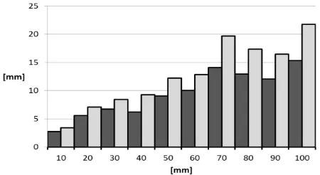
3.2.2 Leica Cyclone 7.1: Leica’s Cyclone software is capable of performing target based registrations, surface based regist-rations, using geometric primitives as well as a combination of all mentioned approaches. Implemented quality measures are a histogram depicting the deviations, a function to colour the registered point clouds differently in order to check the result manually as well as a report that gathers transformation parameters and a statistical description of the residuals. Control parameters of the programme are the number of points that are used to compute the transformation parameters whose default setting is 3% of the points within the overlapping area as well as a maximum search distance. Figure 2 illustrates the impact of the maximum search distance (vertical axis) onto the average deviations and their respective root mean squares (RMS). Expectedly both measures decreased in general with declining search distance.
Figure 2: Influence of maximum search distance onto average deviations (dark grey) and their respective RMS (light grey)
Table 4 gathers the corresponding transformation parameters for three selected settings where the first column “Res.” (Result) depicts the search radius and “Avg. Err.” the average error both International Archives of the Photogrammetry, Remote Sensing and Spatial Information Sciences, Volume XXXIX-B5, 2012
in mm. Nevertheless is the allegedly most accurate result not the closest one to the set of reference parameters. In fact one can’t draw conclusions about a whole set of transformation parameters in this table but only for its single components hence none of the computed sets can be regarded as being the best result.
Table 4: Transformation parameters calculated with Cyclone
Res. tx [m] ty [m] tz [m] rx [°] ry [°] rz [°] Avg.
Err.
10 0.001 0.009 0.019 0.105 0.006 10.622 2.73
50 0.013 0.034 0.020 0.069 -0.034 10.712 9.0
100 0.027 0.051 0.160 0.261 -0.255 10.562 15.3
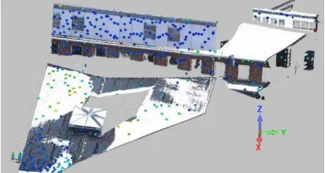
3.2.3 GFaI Final Surface 3.0.5: Final Surface is a software package that has mainly been developed for being used in the field of mechanical engineering. Figure 3 illustrates a colour coded visualisation of 500 points that were used to compute a set of transformation parameters. Small deviations are coloured blue; shades of green describe the medium section while yellow to red represent the large end of the spectrum. It can clearly be seen that the distribution of points is quite heterogeneous. The distribution of points is as usually determined by a random component within the implementation. Nevertheless the likelihood for points of being selected is higher for points that have been captured in areas with high point density which
occurs very likely close to the TLS’s standpoint as visible in
Figure 3.
Figure 3: Colour coded visualisation of all applied tie points
An established approach in surveying to draw meaningful conclusions about the calculated transformation parameters is a regular distribution of tie points in order to ensure verification within a whole dataset as already pointed out by Dold & Brenner (2008) while Rusinkiewicz & Levoy (2001) propose an approach where the variation of normals is as large as possible. A close look at the roof reveals small deviations within the densely covered foreground while the sparse sampled area shows larger deviances. Table 5 gathers results based on 5000 points. Result 1 used the best matching 90% of these points while result 2 applied a margin of 50% leading to an applied amount of 2500 points. It is noteworthy that the individual transformation parameters only slightly change while the average error implies a significant enhancement of the results.
Table 5: Transformation parameters computed with Final Surface
Res. tx [m] ty [m] tz [m] rx [°] ry [°] rz [°] Avg.
Err.
1 -0.012 -0.036 0.196 0.304 -0.033 10.657 19.6
2 -0.009 -0.024 0.189 0.315 -0.015 10.634 5.3
3.2.4 4-Points Congruent Sets Algorithm: The academic 4PCS-algorithm, which was applied with default settings, detected four congruent planes within the deformed scene while 559 points have been used to verify the computed transformation parameters. As 476 points satisfied the acceptable margin of error a quality measure of 85.1% has been computed while Table 6 depicts the respective transformation parameters. Even though the individual transformation parameters show large deviations to the reference values the result was good enough as an initial alignment for the ICP.
Table 6: Transformation parameters calculated by the 4PCS-algorithm
tx [m] ty [m] tz [m] rx [°] ry [°] rz [°]
Avg. Err.
0.009 -0.057 0.061 0.898 0.083 10.349 92.5
3.3 Interpretation of the results
It has been shown that significantly different results have been processed after comparing the outcome of all solutions, as pointed out in 3.1 on example of the “buddha” dataset. None of
the implementations was able to cope with the “snow” dataset
that has been captured with a compensator equipped TLS. This can be constituted by rotational deviations from 0 in x and y -direction as well as large translational variations in vertical direction. None of the implemented quality measures led to the conclusion that the “best” result has been achieved.
4. INTRODUCTION OF NOVEL QUALITY MEASURES
The following section describes a selection of measures that satisfy demands of quality assurance, can furthermore be used to objectively evaluate automated matching processes and finally assess the quality of the applied datasets from the viewpoint of surveying. The majority of proposed quality measures are heavily inspired by approaches that are established in the field of surveying for centuries. A reason why these quality measures are not included in the vast majority of surface matching algorithms can be simply justified by their roots in computer science or more specific in the field of computer vision where the “correctness” of the solution plays a minor role. An analogue issue concerning different point of views between various fields of science is tellingly described by Foerstner (2002). Most of the proposed measures have been implemented in a prototype version of Final Surface.
4.1 Stability
In order to rate the rigidity of a computed set of transformation parameters a stability measure is introduced. Therefore normal vectors from all corresponding points have been computed who are then sorted into a unit sphere which is described by a regular grid consisting of 10° by 10° segments. In a first step the element of the unit sphere with the most entries is determined which describes the most stable direction respectively vector. All other entries are then normalised in relation to this value. The best geometric configuration to this vector would be a plane normally aligned to the reference vector which is why such a plane is computed. In order to determine how well this optimal configuration is satisfied all entries according to their normalised lengths and directions are projected onto this plane while the longest one has to be determined. During the last step of the algorithm a plane is computed that runs through both previously determined vectors while the largest projected vector International Archives of the Photogrammetry, Remote Sensing and Spatial Information Sciences, Volume XXXIX-B5, 2012
is yet to be calculated again. As a result the most dominant direction of the dataset is determined and the relative stability between the individual axes. For the “snow” scene 449 normal
vectors have been segmented in 69 groups. The “strongest”
standardised normal with 55 votes was facing the wall of the building: 0.9984 in x-direction, 0.0159 in y-direction and 0.0247 in vertical direction according to the coordinate system illustrated in Figure 3. Perpendicularly aligned to this vector were 46 sorted vectors leading to a stable ratio of 84% between the two axes. The final vector, roughly aligned in y-direction, can be considered the weakest one with only 13 votes.
4.2 Ratio of Coverage
The relative ratio of coverage rRoC [%] describes a quotient between a surface that is described by two overlapping point clouds and the extent which is delimited by all applied corresponding points and inspired by Otto von Gruber’s (1924) recommended distribution of tie points in photogrammetry. Nevertheless it only describes the maximum used expansion of corresponding points but does not describe the distribution of the applied tie points which is depicted in Figure 3. The common surface from both scans of the “snow” scene measures 217 m² while the area delimited by the corresponding points adds up to 145 m² which leads to an rRoC of 67%. Another important question is how much overlap exists between two point clouds in relation to their respective size. This measure is called minRoC, which stands for minimum ratio of coverage, and can be described by the quotient between the overlapping area and the largest surface from one of the two point clouds. Applied onto the “snow” dataset the minRoC adds up to 98%, as epoch 1 extends to 222 m² while the overlapping area sums up to 217 m², which means that both point clouds nearly overlap entirely.
A simple possibility to visualise the density of corresponding points within the overlapping area is by using the data structure that organises the point clouds. Final Surface applies an octree so that the number of correspondences per cell can be determined. Figure 4 illustrates the point density per octree cell on example of the roof section, see Figure 3, while the façade would be located to the left. The size of the depicted octree cells add up to 3 m in all dimensions and are represented by the blue coloured grid. It can clearly be seen that the distribution of corresponding points does not satisfy geodetic perceptions as some areas are even uncontrolled as depicted by red. If this dataset would be registered based on the current distribution of correspondences instabilities around the x-axis are likely to occur due to the relatively small stable base as illustrated in blue and green.
Figure 4: Colour coded visualisation of the corresponding point density on the roof section
4.3 Reliability of used points
Influencing factors onto the accuracy of measured points have already been mentioned in section 1 and thus have an impact onto the result of a matching process as well. Major impacts are the distance between scanner and an corresponding object point, the incidence angle of the emitted laser beam as well as radiometric properties of the surveyed object that are represented by the intensity value. The last mentioned parameter is influenced by the first two whereas these impacts can be corrected as shown by Wujanz (2009). After this compensation all introduced factors can be used to estimate single point accuracies which could then be applied to evaluate the current sample points or filter data according to certain quality measures to dismiss inadequate information. By deriving individual single point accuracies for all applied tie points the naive assumption of equally accurate points can be dismissed and techniques from the well-established field of weighted least squares adjustment (Helmert, 1872, pp.113) can be applied as pointed out in the following section.
4.4 Quality of the Transformation Parameters
The ICP as well as the 4PCS share the concept of using Euclidian distances between registered point clouds in order to evaluate the outcome. The problem of this approach is that it does not contain expressiveness on how well the sampled points satisfy the functional relationship to derive the transformation parameters. This drawback becomes obvious especially when datasets including deformation have been introduced. Furthermore both solutions dismiss point pairs that lie above a predefined tolerance which means that a sufficient solution can always be found while their standard deviations or RMS would appear to be acceptable even though unsatisfying transformation parameters might have been computed. The only matching approach that is based on the stable fundament of adjustment calculation is Gruen & Akca’s (2005) LS3D algorithm which is capable of coping with different accuracies / weights and delivers quality measures for accuracy as well as reliability. Hence it is currently the most transparent approach in terms of quality assurance and tunable. The only drawback of the mentioned procedure is the need of a quite good initial alignment.
A way to determine the quality of the matching process is by introducing the corresponding points from the last iteration of the ICP into a six parameter transformation adjustment where three translations and three rotations are estimated. In principle the ICP is used to generate point pairs from two datasets while the adjustment determines the transformation parameters and computes their respective standard deviations. As this simple test was only conducted for the last iteration it made no sense to introduce conditions. Conditions, such as fixing the rotations around X and Y axis, are a logical yet needed step as most modern TLS apply a compensator in order to set the vertical Z axis plumb. Table 7 lists the standard deviations (1σ) for all estimated parameters that have been computed based on the last iteration of the ICP for result 1 from Table 5. The standard deviations for the translations appear to be rather small while the ones for the rotational components are relatively high.
Table 7: Standard deviations for the estimated parameters as matched by the ICP
σ
tx [mm]σ
ty [mm]σ
tz [mm]σ
rx [°]σ
ry [°]σ
rz [°]1.67 1.75 1.77 0.645 0.355 0.268
5. CONCLUSIONS AND OUTLOOK
The biggest drawback of all implementations and algorithms is the use of one-dimensional error metrics which does not describe any significance of how well a point satisfies the functional demands of this three-dimensional problem. Furthermore no algorithm is capable to fix certain parameters during the matching process in order to preserve for instance a certain alignment which can even be seen on the reference values in Table 2. While ICP chooses a subset of points for computation and evaluation of the calculated transformation parameters 4PCS uses only a sample for the sake of assessment. The coarse 4PCS approach was capable of bringing the “snow” dataset into a sufficient alignment so that the ICP was able to converge however always to local minima. Neither of both basic algorithms indicated robustness against deformation nor showed their embedded quality measures any interpretable sign for deformation within the computed dataset. A well-grounded comparison of the three ICP-based algorithms is not feasible as no information is given which points have been used (apart from Final Surface) nor which error metric is minimised.
While the introduced quality measures stability and ratio of coverage describe the properties of the data input the quality of the transformation parameters rate the actual outcome of the matching process. It has to be mentioned that the significance of most of these measures is influenced by the distribution of tie points which is why a regular distribution of points should be implemented. Further research will focus on the development of fully controllable, robust and reliable matching algorithms for automatic deformation analysis from TLS point clouds. The problem of dismissing outliers will be tackled by applying several approaches: robust estimators, segmentation of the object space as well as applying the maximum subsample method (Neitzel, 2005) which identifies the largest consistent subsample within the processed datasets in order to receive acceptable residuals from least squares adjustment.
6. REFERENCES
Aiger, D., Mitra, N.J., Cohen-Or, D., 2008. 4-points congruent sets for robust pairwise surface registration. Proceedings of the ACM SIGGRAPH 2008 symposium, New York, United States of America, pp. 1–10.
Bae, K.-H. & Lichti, D. D., 2008. Automated registration of three dimensional unorganised point clouds. ISPRS Journal of Photogrammetry and Remote Sensing, Vol. 63 (1), pp. 36-54.
Besl, P. & McKay, N., 1992. A method for registration of 3D shapes. IEEE Trans. Pattern Anal. Mach. Intell. 14, pp. 239– 256.
Boehler, W., Bordas, V. and Marbs, A., 2003. Investigating Laser Scanner accuracy. In: IAPRS (ed.), Proc. in the CIPA 2003 XVIII International Symposium, Vol. XXXIV(5/C15), Institute for Spatial Information and Surveying Technology, Antalya, Turkey, pp. 696–701.
Boehm, J. & Becker, S., 2007. Automatic Marker-Free Registration of Terrestrial Laser Scans using Reflectance Features. Proceedings of 8th Conference on Optical 3D Measurement Techniques, Zurich, Switzerland, July 9-12, 2007, pp. 338-344.
Chen, Y. & Medioni, G., 1991. Object Modeling by Registration of Multiple Range Images. Proceedings of the Intl. Conf. on Robotics and Automation, pp. 2724-2729, Sacramento, United States.
Dold, C., Ripperda, N., Brenner, C., 2007. Vergleich verschiedener Methoden zur automatischen Registrierung von terrestrischen Laserscandaten. In: Photogrammetrie, Laserscanning, Optische 3D Messtechnik, Oldenburger 3D-Tage 2007, pp. 196-205, Germany.
Dold, C., & Brenner, C., 2008. Analysis of Score Functions for the Automatic Registration of Terrestrial Laser Scans, International Archives of the Photogrammetry, Remote Sensing and Spatial Information Sciences, vol. XXXVII, Beijing, China.
Foerstner, W., 2002. Computer Vision and Photogrammetry – mutual questions: geometry, statistics and cognitions. Bildteknik/Image Science, Swedish Society for Photogrammetry and Remote Sensing, 151-164
Gielsdorf, F., Gruendig, L., Milev, I., 2008. Deformation analysis with 3D laser scanning. Proceedings of the 13th FIG Symposium on Deformation Measurement and Analysis, Lisbon, Portugal.
Gruber, O. von, 1924. Einfache und Doppelpunkteinschaltung im Raum. Verlag Georg Fischer, Jena, Germany.
Gruen, A., Akca, D., 2005. Least squares 3D surface and curve matching. ISPRS Journal of Photogrammetry and Remote Sensing, 59 (3), pp. 151-174.
Helmert, F. R., 1872. Die Ausgleichungsrechnung nach der Methode der kleinsten Quadrate. B.G. Teubner Verlag, Leipzig, Germany.
Neitzel, F. (2005). Die Methode der maximalen Untergruppe (MSS) und ihre Anwendung in der Kongruenzuntersuchung geodätischer Netze. ZfV 130, Nr. 2, pp. 82-91.
Rusinkiewicz, S. & M. Levoy, 2001. Efficient Variants of the ICP Algorithm. Proceedings of the Third Intl. Conf. on 3D Digital Imaging and Modeling, pp. 142-152.
Soudarissanane, S., Lindenbergh, R., 2011, Optimizing Terrestrial Laser Scanning Measurement Set-up. ISPRS Workshop Laser scanning 2011, 29/08/2011, Volume XXXIII, Calgary,Canada.
Wujanz, D., 2009. Intensity calibration method for 3D laser scanners. New Zealand Surveyor, No. 299: pp. 7-13.
7. ACKNOWLEDGEMENTS
The author would like to express his gratitude to Dror Aiger for contributing his 4PCS code. He’d also like to thank Prof. Dr.-Ing. Frank Neitzel for his valuable remarks and Daniel Krueger for his support during data acquisition. This research has been supported by the German Federal Ministry of Education and Research (BMBF) listed under the support code 17N0509.