Quasi-Newton Method for Absolute Value Equation Based on Upper Uniform Smoothing Approximation Function

DOI: _{10.12928/TELKOMNIKA.v14i3.3785}  1134

Quasi-Newton Method for Absolute Value Equation

Based on Upper Uniform Smoothing Approximation

Function

Longquan Yong*, Shouheng Tuo

School of Mathematics and Computer Science, Shaanxi University of Technology, Hanzhong 723001, China

*Corresponding author, e-mail: yonglongquan@126.com

Abstract

Generally, absolute value equation (AVE), Ax - |x| = b, is an NP-hard problem. Especially, how to find all solutions of AVE with multi-solutions is actually a more difficult problem. In this paper, an upper uniform smooth approximation function of absolute value function is proposed, and some properties of uniform smooth approximation function are studied. Then, AVE, Ax - |x| = b, where A is a square matrix whose singular values exceed one, is transformed into smooth optimization problem by using the upper uniform smooth approximation function, and solved by quasi-Newton method. Numerical results in solving some given AVE problems demonstrated that our algorithm is valid and superior to that by lower uniform smooth approximation function.

Keywords: quasi-Newton method, absolute value equation, absolute value function, upper uniform smoothing approximation function, singular value

Copyright © 2016 Universitas Ahmad Dahlan. All rights reserved.

1. Introduction

Consider the absolute value equation (AVE):

Ax

−

x

=

b

(1)

Where

A R

∈

n n× ,

x b

,

∈

R

n, and

x

denotes the vector with absolute value of each component of

x

. Mangasarian O.L et al. shown that AVE (1) is NP-hard in general form. Hence how to solve the AVE directly attracts much attention [1].

Based on a new reformulation of the AVE (1) as the minimization of a parameter-free piecewise linear concave minimization problem on a polyhedral set, Mangasarian [2] proposed a finite computational algorithm that is solved by a finite succession of linear programs. In the recent interesting paper of Mangasarian [3, 4], a semismooth Newton method is proposed for solving the AVE, which largely shortens the computation time than the succession of linear programs (SLP) method. It showed that the semismooth Newton iterates are well defined and bounded when the singular values of

A

exceed 1. However, the global linear convergence of the method is only guaranteed under more stringent condition than the singular values of

A

exceed 1. Mangasarian [5] formulated the NP-hard n-dimensional knapsack feasibility problem as an equivalent absolute value equation in an n-dimensional noninteger real variable space and proposed a finite succession of linear programs for solving the AVE (1).

based on lower uniform smoothing approximation function are proposed in [14, 15]. Yong has applied AVE to solve two-point boundary value problem of linear differential equation [16].

Compared with literature [15], the basic contribution of present work is that an upper uniform smooth approximation function of absolute value function is established. After replacing the absolute value function by upper uniform smooth approximation function, the non-smooth AVE is formulated as smooth nonlinear equations, furthermore, an unconstrained smooth optimization problem, and solved by quasi-Newton method.

Upper uniform smoothing approximation function of absolute value function is given, and its properties are studied in section 2. Non-smooth AVE is formulated as a smooth nonlinear equations, furthermore, an unconstrained smooth optimization problem; meanwhile, some lemmas for AVE that will be used later are given in section 3. Quasi-Newton method to AVE is proposed in section 4. Effectiveness of the method is demonstrated in section 5 by solving some randomly generated AVE problems with singular values of

A

exceeding 1. Section 6 concludes the paper.

All vectors will be column vectors unless transposed to a row vector. For

x

∈

R

n the 2-norm will be denoted by ||x||, while |x| will denote the vector with absolute values of each component of

x

. The notation

A R

∈

n n× _{will signify a real n n× matrix. For such a matrix}

A

T

will denote the transpose of

A

. We write

I

for the identity matrix, e for the vector of all ones (

I

and e are suitable dimension in context). X =diag x{ }i for the diagonal matrix whose

elements are the coordinates

x

_i of n

x∈R .

2. Upper Uniform Smoothing Approximation Function of Absolute Value Function Definition 2.1 A function 1 1

, 0

:

f

_µ

=

R

→

R

µ

> is called a uniformly smoothing approximation function of a non-smooth function 1 1

:

f

=

R

→

R

if, for any

t

∈

R

1_,

f

µ is continuously differentiable, and there exists a constant

κ

such that:

( )

t

( )

t

,

>0

f

µ

−

f

≤

κµ

∀

µ

,

Where κ >0 is constant independent on

t

.

Obviously, absolute value function

φ

( )

t

=

t

is non-smooth. Following we will give a uniformly smoothing approximation function of

φ

( )

t

.

Theorem 2.1 Let

( )

sin

ln e

sin

e

sin

, 0

2

t t

t

µ µ

µ

π

φ

=

µ

⋅







+

−







< <

µ





. Then

(i)

0

<

φ

_µ

( )

t

−

φ

( )

t

≤

sin ln 2

µ

;

(ii) d

(

( )t

)

₁ dt

µ

φ

< , and

(

)

0

( )

0

t

d t

dt

µ

φ

=

= .

Proof (i).

sin sin sin sin sin

( ) ( )=sin ln e e sin ln =sin ln e e

t t t t t

t t

t t µ µ e µ µ µ

µ

φ φ µ µ µ

− − −

− _{ }

 

 

− _ + _− _ + _

   

,

Since

t

= max{ ,

t

−

t

}

, so

t

− ≤ − − ≤

t

0,

t

t

0

. Moreover,

t

−

t

or

− −

t

t

is equal to 0 at

least. Then sin sin

0=sin

ln1

sin

ln e

e

sin

ln(1 1)=sin

ln 2

t t t t

µ µ

µ

µ

µ

µ

− − −









<



+



≤

+





, That is:

(ii)

(

)

2

sin sin sin

2

sin sin sin

( )

e

e

e

1

=

e

e

e

1

t t t

t t t

d

t

dt

µ µ µ

µ

µ µ µ

φ

−

−

−

−

=

+

+

,

Thus,

(

( )

)

1

d

t

dt

µ

φ

<

and

(

)

sin sin

sin sin

0

0

( )

e

e

=0

e

e

t t

t t

t

t

d

t

dt

µ µ

µ

µ µ

φ

−

− =

=





−





= 





+







[image:3.595.106.503.268.759.2]

.

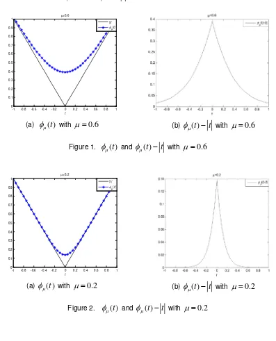
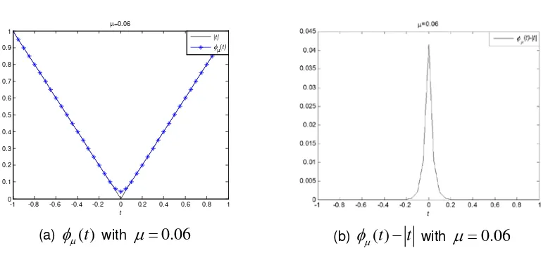
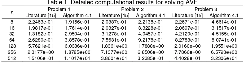
Figure 1-3 show

φ

_µ

( )

t

and

φ

_µ

( )

t

−

t

with

µ

=

0.6,

µ

=

0.2,

µ

=

0.06

.

(a)

φ

_µ

( )

t

with

µ =

0.6

(b)

φ

_µ

( )

t

−

t

with

µ

=

0.6

Figure 1.

φ

_µ

( )

t

and

φ

_µ

( )

t

−

t

with

µ

=

0.6

(a)

φ

_µ

( )

t

with

µ

=

0.2

(b)

φ

_µ

( )

t

−

t

with

µ

=

0.2

Figure 2.

φ

_µ

( )

t

and

φ

_µ

( )

t

−

t

with

µ

=

0.2

-1 -0.8 -0.6 -0.4 -0.2 0 0.2 0.4 0.6 0.8 1

0 0.1 0.2 0.3 0.4 0.5 0.6 0.7 0.8 0.9 1

t

µ=0.6

|t| φµ(t)

-1 -0.8 -0.6 -0.4 -0.2 0 0.2 0.4 0.6 0.8 1

0 0.1 0.2 0.3 0.4 0.5 0.6 0.7 0.8 0.9 1

t

µ=0.2

(a)

φ

_µ

( )

t

with

µ =

0.06

(b)

φ

_µ

( )

t

−

t

with

µ

=

0.06

Figure 3.

φ

_µ

( )

t

and

φ

_µ

( )

t

−

t

with

µ

=

0.06

From Figure 1-3, we can see that

φ

_µ

( )

t

is decreasing with the decrease of parameter

µ

, and

0

lim

_µ

( )

t

( )

t

µ_→ +

φ

=

φ

. So

φ

µ

( )

t

is an upper uniform smooth approximation function of

absolute value function.

3. Smoothing approximation function of AVE

Define

:

n n

H

=

R

→

R

by:

( ) :

H x = Ax− x −b. (2)

H

is a non-smooth function due to the non-differentiability of the absolute value function. In theory,

x

is a solution of the AVE (1) if and only if

H x

( )

=

0

. In this section we give a smoothing function of

H

and study its properties. Firstly we give some lemmas.

Lemma 3.1 [1]

(a) The AVE (1) is uniquely solvable for any

b

∈

R

n if the singular values of

A

exceed 1.

(b) The AVE (1) is uniquely solvable for any

b

∈

R

n if 1

1

A

− < .

Lemma 3.2. For a matrix

A R

∈

n n× , the following conditions are equivalent. (a) The singular values of

A

exceed 1.

(b) 1

1

A

− < .

Lemma 3.3[15]. Suppose that

A

is nonsingular and 1

1

B

A

− < . Then,

A

+

B

is nonsingular.

Lemma 3.4[15]. Let

D

=

diag d

( )

with

d

i

∈

[ 1,1],

−

i

=

1, 2,



,

n

. Suppose that

1

1

A

− < .

Then,

A D

+

is nonsingular.

Definition 3.1[15]. A function

:

n n, 0

H

_µ

=

R

→

R

µ

> is called a uniformly smoothing approximation function of a non-smooth function

H

:

=

R

n →

R

n _{if, for any}

x

∈

R

n_,

H

µ is continuously differentiable, and there exists a constant

κ

such that:

( )x ( )x , >0

H

µ −

H

≤

κµ

∀

µ

.

Where

κ

>

0

is constant without depend on

x

.

-1 -0.8 -0.6 -0.4 -0.2 0 0.2 0.4 0.6 0.8 1 0

0.1 0.2 0.3 0.4 0.5 0.6 0.7 0.8 0.9 1

t µ=0.06

[image:4.595.106.495.74.264.2]

Let

φ

( )

x

=

(

φ

( ), (

x

₁

φ

x

₂

),



, (

φ

x

n

)

)

T,

φ

( )

x

i

=

x i

i

,

=

1, 2,



,

n

.

For any 0

2

π

µ

< <

, let

φ

µ

( )

x

=

(

φ

µ

( ),

x

₁

φ

µ

( ),

x

₂



,

φ

µ

( )

x

n

)

T,

sin sin

( ) sin

ln e

e

,

1, 2,

,

i i

x x

i

x

µ µ

i

n

µ

φ

µ

−





=

⋅





+





=







.

Define

H

:

R

n

R

n

µ

=

→ by:

( )x ( )x

H

µ

=

Ax

−

φ

µ

−

b

. (3)

Clearly,

H

µ is a smoothing function of

H

. Now we give some properties of

H

µ, which will be used in the next section.

By simple computation, for any

µ

>

0

, the Jacobian of

H

_µ at

x

∈

R

n

is:

(

1 2

)

( )x ( ),x (x ), , (x_n)

H

µ′ =

A

−

diag

φµ′ φµ′ φµ′

Where,

sin sin

sin sin

e

e

( )

,

1, 2,

,

e

e

i i

i i x x

i x x

x

i

n

µ µ µ µ µ

φ

− −

−

′

=

=

+



.

Theorem 3.1. Suppose that 1

1

A

− < . Then

H

µ′

( )

x

is nonsingular for any

0

2

π

µ

< <

.

Proof: Note that for any

0

2

π

µ

< <

, by Theorem 2.1,

φ

_µ

′

( )

x

_i

<

1,

i

=

1, 2,



,

n

.

Hence, by Lemma 3.4, we have

H

µ′

( )

x

is nonsingular.

Theorem 3.2. Let

H x

( )

and

H

µ

( )

x

be defined as (2) and (3), respectively. Then,

( )

x

H

_µ is a uniformly smoothing approximation function of

H x

( )

.

Proof: For any

0

2

π

µ

< <

, by Theorem 2.1.

2 1

( )

x

( )

( )

x

( )

ni

( )

x

i

( )

x

i

ln 2 sin

H

µ

−

H x

=

φ

µ

−

φ

x

=

∑

₌

φ

µ

−

φ

≤

n

⋅

µ

.

Denote

x

( )

µ

is the solution of (3), then

x

( )

µ

converges to the solution of (1) as

µ

goes to zero.

For any

0

2

π

µ

< <

, Define

θ

:

=

R

n →

R

_and

:

n

R

R

µ

θ

=

→ by:

2

1 ( )

2

( )

x

H x

θ

=

, ( ) 1 2

2

( )

x

H

x

µ µ

θ

=

.

Theorem 3.3. Suppose that 1

1

A

− < . Then, for any

0

2

π

µ

( )x 0

µ

θ

∇

=

implies that

θ

_µ( )x

=

0.

Proof: For any

0

2

π

µ

< <

and n

x

∈

R

, ( )

[

( )]

T

( )

x

H

x

H

x

µ µ µ

θ

′

∇

=

. By Theorem 3.1,

( )

x

H

µ′ is nonsingular. Hence, if ∇

θ

µ( )x

=

0, then

H

µ

( )

x

and

θ

µ( )x

=

0.

4. Quasi-Newton Method

In this section, we give a quasi-Newton method for solving

H

µ

( )

x

=

0

.

Algorithm 4.1. Quasi-Newton method for AVE. Step 1. Given

0

0

,

0

2

k

π

µ

<

<

=

. Establish the objective function.

2

1 ( )

2 ( )

k x H k x

µ µ

θ = .

Step 2. Apply quasi-Newton method to solve min ( ) k

x

θ

µ x . Let

x

k =arg min_x

θ

µk( )x . Step 3. Check whether the stopping rule is satisfied. If satisfied, stop.

Step 4. Let ₁

(1

k

) /

k

k k

e

e

µ µ

µ

₊

=

µ

+ −

,

k

:

= +

k

1

. Return to step 2.

5. Numerical Results

In this section, some numerical tests are performed in order to illustrate the implementation and efficiency of the proposed method. Throughout the computational experiments, we set

µ

₀

=

sin1

, and initial point

x

0

=

(10, 10,



,10)

T_{, and we set the} random-number generator to the state of 0 so that the same data can be regenerated. All experiments were performed on MatlabR2009a with Intel(R) Core(TM) 4×3.3GHz and 2GB RAM.

5.1. AVE Problems

Problem 1. Let

A

be a matrix whose diagonal elements are 500 and the nondiagonal elements are chosen randomly from the interval

[1, 2]

such that

A

is symmetric. Let

e

I

A

b

=

(

−

)

such that

x

=

(1, 1,



,1)

Tis the unique solution. Problem 2. Let matrix

A

is given by:

, 1 1,

4 ,

,

0.5,

1, 2,

, .

ii i i i i i j

a

=

n

a

₊

=

a

₊

=

n

a

=

i

=



n

Let

b

=

(

A

−

I

)

e

such that

x

=

(1, 1,



,1)

T is unique solution.

Problem 3. Consider some randomly AVE problems with singular values of

A

exceeding 1 where the data (A, b) are generated by the Matlab scripts:

rand('state',0);R=rand(n,n);

A=R'*R+n*eye(n,n);b=(A-eye(n,n))*ones(n,1);

And

x

=

(1, 1,



,1)

Tis the unique solution.

5.2. Computational Results

[image:7.595.100.497.87.190.2]

Table 1.Detailed computational results for solving AVE

n Problem 1 Problem 2 Problem 3

Literature [15] Algorithm 4.1 Literature [15] Algorithm 4.1 Literature [15] Algorithm 4.1

8 2.2463e-01 1.9156e-01 2.0387e-01 2.2138e-01 2.2671e-01 4.6614e-01

16 1.9817e-01 1.7614e-01 2.0327e-01 3.3228e-01 2.0697e-01 3.1517e-01

32 1.3182e-01 2.9504e-01 3.1278e-01 4.0457e-01 4.2120e-01 4.5155e-01

64 2.6280e-01 3.8578e-01 7.5631e-01 9.2178e-01 8.2783e-01 8.0741e-01

128 5.7621e-01 6.0386e-01 1.8361e+00 1.7888e+00 2.0160e+00 1.9551e+00

256 2.3177e+00 1.8785e+00 7.1377e+00 6.8506e+00 7.7866e+00 6.5793e+00

512 1.5106e+01 1.1017e+01 3.8601e+01 3.2385e+01 4.4028e+01 3.2306e+01

From Table 1, with the dimension increased, our method is less time consumed in most cases, especially for larger dimension.

6. Conclusion

A new upper uniform smooth approximation function of absolute value function is presented, and is applied to solve AVE. The effectiveness of the method is demonstrated by solving some randomly generated AVE problems. Future works will also focus on studying the upper uniform smooth approximation function of absolute value function on other engineering problems, such as nonlinear control [17], support vector machines [18-19], artificial intelligence [20].

Acknowledgments

This work is supported by the National Natural Science Foundation of China (11401357), the project of Youth star in Science and technology of Shaanxi Province (2016KJXX-95), and the foundation of Shaanxi University of Technology (SLGKYQD2-14, fckt201509).

References

[1] Mangasarian OL, Meyer RR. Absolute value equations. Linear Algebra and its Applications. 2006; 419(5): 359-367.

[2] Mangasarian OL. Absolute value programming. Computational Optimization and Aplications. 2007; 36(1): 43-53.

[3] Mangasarian OL. Absolute value equation solution via concave minimization. Optim. Lett. 2007; 1(1): 3-8.

[4] Mangasarian OL. A generlaized newton method for absolute value equations. Optim. Lett. 2009; 3(1): 101-108.

[5] Mangasarian OL. Knapsack feasibility as an absolute value equation solvable by successive linear programming. Optim. Lett. 2009, 3(2): 161-170.

[6] C Zhang, QJ Wei. Global and Finite Convergence of a Generalized Newton Method for Absolute Value Equations. Journal of Optimization Theory and Applications. 2009; 143: 391-403.

[7] Louis Caccetta, Biao Qu, Guanglu Zhou. A globally and quadratically convergent method for absolute value equations. Computational Optimization and Applications. 2011; 48(1): 45-58.

[8] Jiri Rohn. On Unique Solvability of the Absolute Value Equation. Optim. Lett. 2009; 3(4): 603-606. [9] Jiri Rohn. A residual existence theorem for linear equations. Optim. Lett. 2010; 4(2 ): 287-292.

[10] Jiri Rohn. An Algorithm for Computing All Solutions of an Absolute Value Equation. Optim. Lett. 2012; 6(5): 851-856.

[11] Muhammad Aslam Noor, Javed Iqbal, Khalida Inayat Noor, Eisa Al-Said. On an iterative method for solving absolute value equations. Optim. Lett. 2012; 6(5): 1027-1033.

[12] Saeed Ketabchi, Hossein Moosaei. Minimum Norm Solution to the Absolute Value Equation in the Convex Case. J. Optim. Theory and Appl. 2012; 154(3): 1080-1087.

[13] Davod Khojasteh Salkuyeh. The Picard-HSS iteration method for absolute value equations. Optim. Lett. 2014; 8(8): 2191-2202.

[14] Longquan Yong, Sanyang Liu, Shouheng Tuo, Kai Gao. Improved harmony search algorithm with chaos for absolute value equation. TELKOMNIKA Telecommunication Computing Electronics and Control. 2013; 11(4): 835-844.

[16] Longquan Yong. Iteration Method for Absolute Value Equation and Applications in Two-point Boundary Value Problem of Linear Differential Equation. Journal of Interdisciplinary Mathematics. 2015; 18(4): 355-374.

[17] Jingqing Han. Using Sign Function and Absolute Function to Construct Nonlinear Function. Control Engineering of China. 2008; 15(S1): 4-6.

[18] Yaxun Wang. Research on 1st-order smooth function of support vector machines and its approximation accuracy. Computer Engineering and Applications. 2008; 44(17): 43-44.

[19] Nengshan Feng, Jinzhi Xiong. The approximation accuracies of polynomial smoothing functions for support vector regression. CAAI Transactions on Intelligent Systems. 2008; 8(3): 266-270.