ISSN: 1693-6930
accredited by DGHE (DIKTI), Decree No: 51/Dikti/Kep/2010 564
Time of Arrival
and
Angle of Arrival
Statistics for Distant
Circular Scattering Model
Guo Limei*1, Nian Xiaohong2 1,2
School of Information Science and Engineering, Central South University Changsha, Hunan, China, +86 73185324179
e-mail: [email protected]*1
Abstrak
Model hamburan umum adalah proses hamburan lokal diasumsikan bahwa stasiun bergerak terletak di dalam wilayah hamburan. Untuk mempelajari model hamburan jauh di lingkungan propagasi pinggiran kota atau berbukit, sebuah modus hamburan melingkar jauh secara statistik berdasarkan geometri di lingkungan sel makro diusulkan. Ekspresi bentuk tertutup dari fungsi kepadatan probabilitas gabungan dari waktu kedatangan/sudut kedatangan, kepadatan fungsi probabilitas marjinal sudut kedatangan dan sudut keberangkatan, kepadatan fungsi probabilitas marjinal waktu kedatangan diturunkan. fungsi kepadatan probabilitas ini memberikan wawasan ke dalam sifat dari model hamburan saluran spasial jauh.
Kata kunci: model hamburan jauh, sudut datang, sudut keberangkatan, waktu datang
Abstract
General scattering model is local scattering process assumed that the mobile station is located inside the scattering region, in order to study distant scattering model in suburban or hilly propagation environment, a geometrically based statistical distant circular scattering mode in macrocell environment was proposed, the closed-form expressions of the joint probability density function of the time of arrival /the angle of arrival, the marginal probability density function of the angle of arrival and the angle of departure, the marginal probability density function of the time of arrival were derived, this probability density function’s provided insight into the properties of the spatial distant scattering channel model.
Keywords: distant scattering model, the angle of arrival, the angle of departure, the time of arrival
1. Introduction
Nevertheless, Most of the existing geometric channel models take into account only the local scattering, the mobile station is located inside the scattering region, and few available models define the shape and distribution of distance scattering. Distance scattering is the scattering process which results from the dominant distant scattering structures far from both the BS and the MS, this type of scattering can occur in hilly and suburban areas due to large scattering structures such as mountains and high building clusters, which have a significant influence on the mobile channel[11]. The contributions of this paper is to study a distant circular scattering model, and derive the joint and marginal probability density functions of the angle of arrival and the time of arrival (TOA) in closed form for distant scattering in macrocell environment, which are required to test adaptive array algorithms for cellular applications..
2. Distant Circular Scattering Model
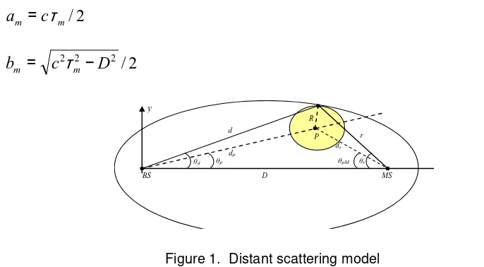
Figure1 shows the proposed distant circular scattering geometry model in macrocell environment, it is assumed that the signals received at BS have interacted with only a single scatterer in the channel, the MS is located on the x-axis with the origin at BS, D denotes the distance between MS and BS, a point P is the centre of the distant scattering circular with a radius R and is denoted by the polar coordinates (dp,θp) and (dr,θr) with respect to the polar coordinates with the origin at BS and MS respectively, the model assumes that the scatterers are uniformly distributed within the circular, a random scatterer position S(xs,ys) can denoted by (d,θd) and (r,θr) with respect to the polar coordinates with the origin at BS and MS respectively,
it is assumed that the distant scattering circular is located inside the ellipse with foci at BS and MS, its semimajor axis am and semiminor axis bm values are given by:
2
/
m
m
c
a
=
τ
(1)2
/
2 2 2
D
c
b
m=
τ
m−
(2)Figure 1. Distant scattering model
Where τm is the maximum delay associated with scatterers within the ellipse. As shown
in Figure1, scatterers were assumed to be uniformly spread over the distant circular, the scatter density function in rectangular coordinates can be written as:
≤
=
otherwise
R
y
x
R
y
x
f
s ss s y xs s
0
|
)
,
(
|
1
)
,
(
2,
π
(3)The total path propagation delay is given by
r
d
c
=
+
τ
(4)Looking at the triangle∆(MS,BS,S)as shown in Figure1, the following equation can be
deduced:
) cos( 2 2 2
d
dD D d d
c
θ
τ
− = + − (5)Squaring both sides of(5)and solving for d results in
BS MS
P d
r R
θd θr
dp
θp θpM
dr
D
) cos ( 2
2 2 2
c D
c D d
d
τ
θ
τ
− −= (6)
Therefore, the location of the scatterer in the rectangular coordinates is given by;
) cos ( 2
cos ) (
cos
2 2 2
c D
c D d
x
d d d
s
θ
τ
θ
τ
θ
− − =
= (7)
) cos ( 2
sin ) (
sin
2 2 2
c D
c D d
y
d d d
s
θ
τ
θ
τ
θ
− − =
= (8)
2.1. Joint TOA/AOA pdf at BS
Once the scatterer distributionfx,y(xs,ys)
s s
and the relations between (xs,ys) and (τ,θd) are
known, the join TOA/AOA pdf ,
(
,
d)
d
f
τθτ
θ
can be obtained by a Jacobian transformation between (xs,ys) and (τ,θd) :b s
b s
s s
s s y x
d x y
y x
y x f f
s s d
θ
θ
τ
τ
θ
τ
θ τ∂ ∂ ∂
∂ ∂
∂ ∂ ∂
= ( , )
) ,
( ,
, 3
2 2 2 2 2 2 ,
) cos ( 4
) cos 2 )(
( ) , (
c D
c c
D c D c D y x f
d
d s
s y
xs s
θ
τ
θ
τ
τ
τ
− − + −
⋅
=
3 2
2 2 2 2 2 2
)
cos
(
4
)
cos
2
)(
(
c
D
R
c
c
D
c
D
c
D
d
d
τ
θ
π
θ
τ
τ
τ
−
−
+
−
=
(9)2.2. AOA pdf at BS
The AOA pdf could be found by integrate the polar coordinate system representation of the scatterer density functionfd,θd(d,
θ
d) with respect to d over the range d1 to d2, where d1 and d2are two pairs of roots for the equations defining the distant scattering discs, in polar coordinates:
]
,
0
[
)
cos(
2
22 2
R
dd
d
d
+
p−
pθ
d−
θ
p∈
(10)Equate (10) to its upper limit of R2producing the following two roots
}
)
(
sin
)
cos(
{
,
2 2 2 21
d
d
p d pR
d
p d pd
=
θ
−
θ
±
−
θ
−
θ
(11)When the relations between (xs,ys) and (d,θd) are known, the joint pdf ( , )
, d
d d
f
d
θ
θ can be
obtained by another Jacobian transformation between (xs,ys) and (d,θd):
)
sin
,
cos
(
)
,
(
)
,
(
,sin cos ,
, s s d d
d s
d s s
s
d
x
y
df
d
d
d
y
d
x
y
x
f
d
f
x yd y
d x b s
b s
s s
s s y x d
d
θ
θ
θ
θ
θ
θ θ
θ
=
∂
∂
∂
∂
∂
∂
∂
∂
=
= =
(12)
Therefore the AOA pdf at BS equals
2 2 1 2 2 2
,
2
1
)
,
(
)
(
21 2
1
R
d
d
dd
R
d
dd
d
f
f
dd d
d
d d
d d
d
θ
θθ
π
π
+
≤
≤
−
−
−
−
=
otherwise
o
d
R
d
R
R
d
R
d
p p d p p p d p p d parcsin
arcsin
)
(
sin
)
cos(
2
2 2 2 2θ
θ
θ
π
θ
θ
θ
θ
(13)2.3. TOA pdf at BS
To identify the support region of θat a specificτ, there exists a τ-constant spatial ellipse
focusing at the base station’s and the mobile station’s spatial locations, any propagation path must bounce off a scatterer lying on this ellipse’s rim, this elliptical rim intersects with the circle (within which the scatterers lie) at two points at most[12], that is θ satisfying the following relation
for a specific time delay τ:
2 2 2 2 2 2 2 2 2
)
cos(
)
cos
(
)
(
)
)
cos
(
2
(
R
c
D
d
c
D
d
c
D
c
D
p d d p p d=
−
−
−
−
+
−
−
θ
θ
τ
θ
τ
τ
θ
τ
(14)In order to simplify calculations, we use another method, in rectangular coordinates the intersection points(x,y) satisfy the following both equations:
=
+
−
=
−
+
−
1
)
2
/
(
)
(
)
(
2 2 2 2 2 2 0 2 0b
y
a
D
x
R
y
y
x
x
(15)Where
x
0=
d
pcos
θ
p,
y
0=
d
psin
θ
p,
a
=
τ
c
/
2
,
b
=
c
2τ
2−
D
2/
2
, after some elementary but rather tedious calculation, equation (15) can be expressed as:
a
tx
4+
b
tx
3+
c
tx
2+
d
tx
+
e
t=
0
(16)where: 2 0 2 2 2 0 2 2 0 4 2 0 2 0 2 0 2 4 0 2 2 0 4 2 2 2 2 4 4 4 2 2 2 4 2 4 2 2 2 0 2 2 0 2 2 2 2 4 3 4 2 4 2 0 0 0 2 2 0 2 2 2 2 0 2 0 2 2 0 2 2 0 3 2 2 2 2 2 2 4 4 2 2 4 2 0 2 2 0 2 2 2 0 2 2 0 2 2 2 0 2 4 4 2 0 2 0 2 2 4 4 2 2 2 2 2 2 2 2 16 2 2 2 2 2 2 2 4 4 2 4 2 4 2 2 2 3 2 4 2 6 2 2 2 2 2 4 4 2 1 2 a x D b x b x R x y x R y R y a D b R a b D R b a b D b a D b y b y e a b DR a D b a Db R x x y a x b D a Db y x b a x Db x d a D b a b R a b D a b a x Db b x a b y a x b R y c a Db a x b x a Db b a b a b a t t t t t − + + − + + − + + + − − + + − = − − + + − + − − + − = − + + − − + + + − − = − + − = + + − =
Equation (16) is a quartic equation, the quartic can be solved by means of a method discovered by Lodovico Ferrari[14], and its two roots satisfying the following relationships are the solution to the equation (15), we express the roots as x1,x2 and x1≤x2:
d
pcos
θ
p−
R
≤
x
1≤
x
2≤
d
pcos
θ
p+
R
(17)1 2 2 1 2 2
2
)
/
)
2
/
(
(arctan
x
a
D
x
b
b
d−
−
=
θ
(18)2 2 2 2 2 2
1
)
/
)
2
/
(
(arctan
x
a
D
x
b
b
d−
−
=
θ
(19)In addition, the minim and maximum AOA for distant scattering are given by:
p
p d
R
arcsin 1
min =θ −
θ (20)
p
p d
R
arcsin
1
max =
θ
+θ
(21)using ) cos ( 2 2 2 2 c D c D d d τ θτ − −
= ,
θ
d=θ
max1,and 2 2R
d
d
=
p−
,we can obtain the upper limit of τ:c d R R d D D R d R
dp2 2 2p 2 2 2 ( 2p 2)1/2cos( p arcsin( / p))
max + − − + − + − =
θ
τ
(22)For the same reason, the lower limit of τis:
c d R R d D D R d R
dp p 2 ( p ) cos(p arcsin( / p))
2 / 1 2 2 2 2 2 2 2 min − − − + − + − =
θ
τ
(23)Therefore the pdf of TOA at BS can be found as:
≤
≤
−
−
+
−
==
∫
otherwise
d
c
D
R
c
c
D
c
D
c
D
f
d d d d d0
)
cos
(
4
)
cos
2
)(
(
)
(
max min 3 2 2 2 2 2 2 2 2 1τ
τ
τ
θ
τ
θ
π
τ
τ
θ
τ
τ
θ θτ (24)
Using the following transformations:
2 2 2 2 1 2 , 1 2 sin , 1 1 cos , 2 tan t dt d t t t t
t d d d
d + = + = + − = =
θ
θ
θ
θ
The TOA’s marginal density explicitly depends on the model parameters of R and D:
Where:
D
c
D
c
a
+
−
=
τ
τ
4 ,
2 2 2 2
2 2 2
1
4
2
D
c
R
cD
c
c
a
−
−
=
τ
π
τ
,)
(
4
2
2 2
c
D
D
R
c
a
τ
π
+
=
,2 2
2 3
)
(
2
)
(
c
D
D
R
c
c
D
a
τ
π
τ
+
−
=
2.4. The Angle of Departure (AOD) pdf at MS
The same equations apply at the mobile when scatter density is referred to the polar coordinate system (r,θs) defined at the mobile, the relationship between r and τ is identical in
form to the relationship between d and τ, that is:
)
cos(
2
2 2r
rD
D
r
r
c
θ
τ
−
=
+
−
(26)Squaring both sides of (26) and solving for r results in
)
cos
(
2
2 2 2
c
D
c
D
r
r
τ
θ
τ
−
−
=
(27)Therefore, the location of the scatterer in the rectangular coordinates is also given by:
)
cos
(
2
cos
)
(
cos
2 2 2
c
D
c
D
r
x
r r r
s
θ
τ
θ
τ
θ
=
−
−
=
(28))
cos
(
2
sin
)
(
sin
2 2 2
c
D
c
D
r
y
r r r
s
θ
τ
θ
τ
θ
−
−
=
=
(29)Once the scatterer distribution
f
xs,ys(
x
s,
y
s)
and the relations between (xs,ys) and (τ,θr) are
known, the join TOA/AOD pdf , (, r)
r
fτθ τθ can be obtained by a Jacobian transformation:
3 2
2 2 2 2 2 2
, ,
) cos ( 4
) cos 2 )(
( )
, ( )
, (
c D
R
c c D c D c D y x
y x
y x f f
r
r
r s
r s
s s
s s y x
r s s
r
π
θ
τ
θ
τ
τ
τ
θ
θ
τ
τ
θ
τ
θτ = − + −−
∂ ∂ ∂
∂ ∂
∂ ∂ ∂
= (30)
The AOD pdf at the MS could be found by integrate the polar coordinate system representation of the scatterer density functionfr,θr(r,θr) with respect to r over the range r1 to r2,
where r1 and r2 are two pairs of roots for the equations defining the distant scattering discs when the scatterer density is referred to the polar coordinate system (r,θs), in polar coordinates:
]
,
0
[
)
cos(
2
22 2
R
rd
d
r
+
r−
rθ
r−
θ
pM∈
(31)Equate (31) to its upper limit of R2producing the following two roots
}
)
(
sin
)
cos(
{
,
2 2 2 21
r
d
r r pMR
d
r r pMr
=
θ
−
θ
±
−
θ
−
θ
(32)The joint pdf fr,θr(r,
θ
r) can be obtained by another Jacobian transformation with therelations between (xs,ys) and (r,θr) are known:
) sin , cos ( )
, ( ) ,
( ,
sin cos ,
, x y r r
r y
r x r s
r s
s s
s s y x r
r x y rf r d
r y r x
y x f r f
s s
r s
r s s
s
r θ θ
θ θ θ
θ θ
θ =
∂ ∂ ∂ ∂ ∂
∂ ∂ ∂ =
= =
Therefore the AOD pdf at MS equals
+ ≤ ≤ −
− −
−
=
=
∫
otherwise d
R d
R for
R d R d
otherwise dr r f f
r pM
r r pM
pm r r pM
r r
r r
r r
r r
r
0
arcsin arcsin
) (
sin )
cos( 2
0
) , ( )
(
2
2 2 2
,
2
1
θ θ θ
π
θ θ θ
θ θ
θ θ
θ
(34)
3. Results and Analysis
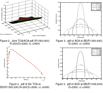
[image:7.595.87.439.110.190.2]In this section the above theoretical models are validate using simulation, the distance between MS and BS is 2km, and its centre is P(1500,400) m, τc=2450m, the joint pdf of TOA/AOA at BS for the uniformly distribution scatterer model is shown in Figure 2 (equation (9)), the radius of cell R is chosen as 200m, equation (13) is plotted in Figure 3, the scatterers are uniformly located within a circles of different radius, equation (25) is plotted in Figure 4, equation (34) is plotted in Figure 5, the pdf derived in this section can be used to simulate a power-delay-angle profile and to quantify angle spread and delay spread[13] for the given R, D and the centre of the scattering circle.
Figure 2. Joint TOA/AOA pdf (P(1500,400); R=200;D=2000; τc =2450)
Figure 3. pdf of AOA at BS(P(1500,400); D=2000;τc =2450)
Figure 4. pdf of the TOA at BS(P(1500,300);R=200;D=2000;τc =2400)
Figure 5. pdf of AOD at MS(P(1500,400); D=2000;τc =2450)
4. Conclusion
In this paper, we have derived geometrical channel model assumed that the scatterers are within a circle far from both BS and MS, this type of scattering can occur in hilly and suburban areas due to large scattering structures such as mountains and high building clusters, which have a significant influence on the mobile channel, the joint TOA/AOA and marginal TOA ,AOA and AOD pdf’s for the circular scattering model are derived.
20 30
40 50
60
3000 3100 3200 3300 3400 3500
4 6 8 10 12 14
x 104
angle of arrival (degree) Time of arrival(sec*c)
J
o
in
t
p
ro
b
a
b
ili
ty
d
e
n
s
it
y
6 8 10 12 14 16 18 20 22 24 0
0.05 0.1 0.15 0.2 0.25 0.3 0.35
AOA(degree)
p
ro
b
a
b
ili
ty
d
e
n
s
it
y
R=50 R=100 R=150 R=200
6.7 6.8 6.9 7 7.1 7.2 7.3 7.4 7.5 7.6 x 10⁻⁶ 3
4 5 6 7 8 9 10 11 12x 10
5
TOA(sec)
p
ro
b
a
b
ili
ty
d
e
n
s
it
y
20 25 30 35 40 45 50 55 60
0 0.02 0.04 0.06 0.08 0.1 0.12 0.14 0.16
AOA(degree)
p
ro
b
a
b
ili
ty
d
e
n
s
it
y
[image:7.595.97.497.320.681.2]Acknowledgments: This work was supported by National Natural Science Foundation of China under Grant Nos. 61075065,60774045
References
[1] Khan N.M, Simsim M.T, Rapajic, P.B. A Generalized Model for the Spatial Characteristics of the Cellular Mobile Channel. IEEE Trans. Vehicular Technology. 2008; 57(1): 22-37.
[2] Seung-Hyun Kong. TOA and AOD Statistics for Down Link Gaussian Scatterer Distribution Model. IEEE transactions on wireless communications. 2009; 8(5): 2609-2617.
[3] M Alsehaili. Angle and time of arrival statistics of a three dimensional geometrical scattering channel model for indoor and outdoor propagation environments. Progress In Electromagnetics Research. 2010; 109 :191-209.
[4] Hamalainen, J. Savolainen, S. Wichman, R. Ruotsalainen, K. Ylitalo, J. On the Solution of Scatter Density in Geometry-Based Channel Models. IEEE Trans. wireless communications. 2007; 6(3):1054-1062.
[5] Vue Ivan Wu, Kainam Thomas Wong. A Geometrical Model for the TOA Distribution of Uplink/Downlink Multipaths,Assuming Scatterers with a Conical Spatial Density. IEEE Antennas and Propagation Magazine. 2008; 50(6):196-205.
[6] Tetsuro Imai, Tokio Taga. Statistical Scattering Model in Urban Propagation Environment. IEEE Trans. Vehicular Technology. 2006; 55(4):1081-1093.
[7] Janaswamy, R. Angle and time of arrival statistics for the Gaussian scatter density model. IEEE Trans.Wireless communications. 2002; 1(3): 488-497.
[8] L. Jiang S. Y. Tan. Geometrically based statistical channel models for outdoor and indoor propagation environments. Journal IEEE Transactions on Vehicular Technology. 2007; 56(6):3586–3593
[9] K N le. A new formula for the angle-of-arrival probability density function in mobile environment. Journal Signal process. 2007; 87(6):1314-1425
[10] Syed Junaid Nawaz, Bilal Hasan Qureshi, Noor M Khan. A Generalized 3-D Scattering Model for a Macrocell Environment With a Directional Antenna at the BS. IEEE Transactions on vehicular technology. 2010; 59(7): 3193-3204.
[11] Khan N M, Islamabad Simsim M T, Rapajic P B. A Generalized Model for the Spatial Characteristics of the Cellular Mobile Channel. IEEE Transactions on Vehicular Technology. 2008; 57(1): 22-37.
[12] Yue Ivan Wu, Wong K T. A geometrical model for the toa distribution of uplink/downlink multipaths. Assuming scatterers with a conical spatial density. IEEE Antennas and Propagation Magazine. 2008; 50(6):196 – 205.
[13] Petrus P, Reed J H, Rappaport T S. Geometrically based statistical channel model for macrocellular mobile environments. IEEE Transactions on Communications. 2002; 50(3): 495-502