A Neural Network Architecture for Statistical Downscaling Technique: A Case Study in Indramayu District

(1)

A Neural Network Architecture for Statistical Downscaling Technique:

A Case

Study in Indramayu District

Agus BuonozyxwvutsrqponmlkjihgfedcbaZYXWVUTSRQPONMLKJIHGFEDCBAl

,Akhmad Faqih3, Rizaldi Boer', I Putu Santikayasa", Arief Ramadharr', M. Rafi Muttqien", M. Asyhar A7. 1,2,3)Centerfor Climate Risks and Opportunity Management in Southeast Asia and Pacific (CCROM-SEAP) Bogor

Agriculture University, Bogor-West Java, Indonesia

4)Departmentof Geophysics and Meteorology, Faculty of Mathematics and Natural Sciences, Bogor Agricultural University, Bogor-West Java, Indonesia

5,6,7)Departmentof Computer Sciences, Faculty of Mathematics and Natural Sciences, Bogor Agricultural University, Bogor-West Java, Indonesia

pudesha@yahoo.co.id, rizaldiboer@gmail.com

ABSTRACT

This research is focused on the development of statistical downscaling model using neural network technique to predict SOND rainfall in Indramayu. SST and rainfall data from multimodel ensemble outputs (derived from 18 ensemble members of ECHAM5 model under SRES AIB scenario) is used as predictor to predict SOND rainfall in each station. SST domains were selected by using cluster and correlation analyses, which were divided into three sets, namely SST lag I (August), lag 2 (July), and lag 3 (June). The Artificial Neural Network (ANN) employed in this study was multilayer perceptron with hidden layer as many as 5, 10,20, and 40, and was trained with back propagation. The results show that the observed value lies between the maximum and minimum values of the predicted data. It is shown that the lagged SST provides better relationship with the observed data, and the optimum number of hidden neurons in neural networks is 5. Maximum correlation resulted from the models is 0.796 with an average of about 0.6. It is found that the prediction results tend to overestimate low rainfall and underestimat~ high rainfall found in the observed data.

Keywords:zyxwvutsrqponmlkjihgfedcbaZYXWVUTSRQPONMLKJIHGFEDCBAGeneral Circular Madel (GeM), Statistical

zyxwvutsrqponmlkjihgfedcbaZYXWVUTSRQPONMLKJIHGFEDCBA

D o w n sca lin g fS lr), Neural Network(NN), Principle Component Analysis (PCA).

I. INTRODUCTION

Facts indicated that climatic conditions could contribute significantly to agricultural productions. In this case, many techniques have been developed to predict climate variables that can be used to support agricultural management system. Most of these techniques support the analysis of climatic effects on a particular region.

In developing the prediction models, there are usually two main obstacles, first is the limitation of historical climate data with a sufficiently long series, and second is the need of future climate projections (under certain scenarios) to study the impacts of climate change. General Circulation Model (GCM) provides a solution to this problem and the data has been widely used for climate change studies. However, due to its coarse resolution, that is about 2x2 degrees, or about 200x200 Ian, the model is unable to capture local variability that is needed in the analysis of a smaller coverage area, such as district level. Therefore there is a gap between the GCM output and the observed data. In this case, the GCM is only able to capture the pattern of average, whereas variability mainly influenced by local fuctors is not accommodated.

This research is addressed to develop a statistical downscaling model using artificial neural networks (ANN). This model links the rainfa!! data from GCMs and Sea Surface Temperature (SST) with the observational data to predict rainfall intensity in indramayu district. Downscaling techniques will be applied to estimate the total rainfall on SOND (September, October, November, and December) season. With 24 time periods of data, an S-fold cross validation technique is implemented to evaluate the model.

The remainder of this paper is organized as follows: Section 2 presents the principles of statistical downscaling. Section 3describes the methodology used in this study Result and discussion is presented in Section 5, and finally, Section 6 is addressed to the conclusions of this research study.

II. STATISTICAL DOWNSCALING

Downscaling is defined as an effort to connect between global-scale (explanatory variables) and local scale climate variables (response variables), [ I]. Figure I illustrates the process of downscaling.

There are two approaches for downscaling, using regional data (obtained from a regional climate model, RCM), or global data (obtained from the general circulation models, GCM). The first approach is known as statistical dynamical downscaling, while the second is known as statistical downscaling (SD). Statistical downscaling based on the relationship between coarse-scale grid (predictor) with local-scale data (response) is expressed with a statistical model that can be used to translate a global scale anomalies which became an anomaly of some variables of local climate (Zorita and Storch 1999, in [2]). In this case the SD is a transfer function that describes the functional relationship of global atmospheric circulation with elements of the local climate, which is formulated as follows:

(2)

where:

Y : response climate variables

X : global climate variables (provided by GCM) t : time period

p : dimension ofY q : dimension of X s : layers in the atmosphere

g : GCM domain

Predictor variable

[image:2.602.47.292.66.421.2]

(Respond variable)

Figure 1. Illustration of the downscaling (Source: [3])

In general SD model involving time series datazyxwvutsrqponmlkjihgfedcbaZYXWVUTSRQPONMLKJIHGFEDCBA(t) and spatial data ofGCM (g). Number ofY, X variables, the layer

of the atmosphere in the model and the autocorrelation and co-linearity on the variables Y and X indicate the complexity of the model. Until now the SD models that have been developed are generally categorized into five, i.e., i) based on regression techniques or classification, ii) based on linear or non linear model, iii) based on parametric and non parametric, iv) based on projection and selection, and v) based on model-driven or data-driven techniques. Nevertheless, an SD model can be included in the combination of the five categories, for example PCR (principle component regression) that were categorized as regression-based methods, linear, parametric, projections and data-driven. In this research, we developed an adaptive neural network (ANN) model for statistical downscaling using data from the GeM and sea surface temperature as explanatory variables. The use of SST data is specifically intended to capture the EI Nino phenomenon, so the model is expected to produce better prediction results.

III. DATA AND EXPERIMENTAL SETUP

A. Data

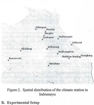
[image:2.602.310.511.189.413.2]

The research involved three types of data, i.e. i) prectpitauon data from GCM model (with the AIB scenario ECHAM5 model (with 18 members and 2.8°x2.8~ resolution), ii) SST data (with 2°x2° resolution) and iii) rainfall data from 17 rain gauge stations in Indramayu, All datasets have the time period from 1979 to 2002 (24 periods). Figure 2 give the spatial distribution of the stations in Indramayu District.

Figure 2. Spatial distribution of the climate station in Indramayu

B. Experimental Setup

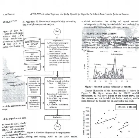
Figure 3 shows five stages of the experimental setup used in this study, i.e.:

a. Preprocessing: This process consists of (I) checking the rainfall observation data (validity and consistency) using the method described by [4]; (2) calculating the SOND season climate variables (rainfall observation of all stations, GCM for all ensemble members). Especially for the S81', the data is divided into three months, i.e. June (lag 3), July (lag 2) and August (lag 1); and (3) calculating the normalization of SOND data for rainfall observations and GCM data, and the normalization of SST for each lag.

b. SST domain selection: clustering the SST do'main into N clusters, and checking the correlation between the normalized observation rainfall with the center of the SST cluster. In this case, the SST data in particular grid is taken as part of the SST domain set if the correlation is found to be statistically different from zero at 0.9 confidence level.

(3)

HAL SETUP l5. After that, 25 dimensional vector GCM is reduced by i.ingprinciple component analysis.

types of data, i.e. I (with the AIB scena! embers and 2.8°~

.2zyxwvutsrqponmlkjihgfedcbaZYXWVUTSRQPONMLKJIHGFEDCBA0x2° resolution),

~---ze stations in ;d from 1979 to ;patial distribution

Prf"1PCOC(!-.i.1i :

1 . (\')'(x:;kt~ni!:Yc-h:ckl.r..,g "for

each mi.nfa.ll s.w.ti:an 2. C(lln7"'~ thl:pr~.iphatk)n

fur SOND{Ob",,.,.,,,i.on "nd (;C>,I daill) . .3. Narm~li7..atkln far the

"h>::,vatkm fahltnlJ. GeM

~J1d"STeaL1 ("'lbt~<.td the value bvtheir S".,..cra~~ II.!>rl<livim h:.·tk~d

de'~·iatkl:n).

I::xpe.rim.nt: !. Neural nct\Vmk mndeli.n2

"inpt.1. SSTdu~'t~:;-...

.deeM ~l1q:r~t ob$:'f\':atlonal

rabfulllbr each statlon '2. nuntb:r of hidd~.n'!)c:llron :

5, W, 20t.and«:t

3. !all o(ssr,!as 3 {June), Ia S 1 (July}. !all ! l.Ausun)·

4, Validation :8-Fold ere ss

of the experimental setu]

-ssconsists of (I). checki validity and consIstency) [4]; (2) calculating t?e :

(rainfall observabOI1;.Figure 3. The flow diagram of the experiments

emble members). Espec~a . . .

1 d . to three months, i.edeling and testmg ANN: In this ANN model, e d I~ gust (lag I)' ruinputsare GCM and SST data, while the outputs are a~ U ND data for1rainfall data of all stations. The developed ANN iuon of SOh lizalel is the multilayer perceptron with one input layer, data, and t e norma hidden layer and one output layer. Input layer '. . lists of two groups of neurons, i.e. one group for lustering the SST domallli_{and another group for rainfall from GCMs, The}

the correlation betwerut layer is in accordance with a consistent number ~infall with the cent~ of tations. T~ining of~he ANN mod~1is based on error . SST data in particular;. propagation ~Igo~thm as .descnbed by [5). Two e . t if the corre}ldered factorsIIIthis experiment are the number of

r

do~1ll set from zero en neurons (i.e.: 5, 10, 20, and 40), and the lag time By dlfferen e SST data, i.e. the SST in June (lag 3), July (lag 2), . August (lag I). By considering that the total period r each rainfall statlO~ th\ta is 24, the 8-fold cross validation is then used to ,redictor is within the dlmebe model,

e. Model evaluation: the ability of neural network techniques in predicting the total rainfall was evalo/l!7gby

.

zyxwvutsrqponmlkjihgfedcbaZYXWVUTSRQPONMLKJIHGFEDCBA

~ $L j\_ ..• • ...c .

"- .,

[image:3.600.46.526.15.491.2]

15

[image:3.600.49.304.58.471.2]

Figure 4. Pattern F statistic values for 17 stations. Clearer illustration of the inconsistencies is shown in Figure 5. The figure shows that the SOND rainfall inconsistent in 1993-1994. Based on the results above, the four stations are not included for further analysis, which mean that only 13 stations will be analyzed in this study.

I.

S7g.I~nUS4-w.~1

•

"

•

zyxwvutsrqponmlkjihgfedcbaZYXWVUTSRQPONMLKJIHGFEDCBA

." .i-«

~

zyxwvutsrqponmlkjihgfedcbaZYXWVUTSRQPONMLKJIHGFEDCBA

...

.

..

/

-.

.

2 0 0

~ 100

••

•

O + - - - , - - - ~ - - ~ - - ~ - - ~ ~ ~

1975 1980 1985 1990 HISS 2000 2005

Y41t

[image:3.600.331.516.363.524.2]

(4)

5x5. After that, 25 dimensional vector GCM is reduced by using principle component analysis.

I'npr<>Cl!"':

Cnr.,:,~'istencych:cki.n,g fhr

each

r.ai.d;'l:j.!I station

2.

('01"l''*'

11.; pr~dpitation

for SOND(Ob$nution "nd(;eMdata}. 3, Nmmaiizatkm for tr:t

observancn r.hlf.IL OeM

ami S.sTdal1l (SiUb!~dc.d

th:, v~I1J..:bytheir H'.,-~N1,g-:

annrl ivide bythe ;;t>In±rrd &,'~~iation).

selection rar each sta don bv

t5lD.2 i.:-me,a~

algdriL'mland mr.relatioo

analysis eaeh starien

2. n'un:ib:r ofb~,n DOLll"W :

5, 10, W, and 4Q .1.ms,,(SS'tdagl{1=),

lasl{juiy). las 1

tAuSUS!l.

4. Validation ;8·f'<>ld cress ,~Ihbtkm

rain-full fer

Figure 3. The flow diagram of the experiments

d. Modeling and testing ANN: In this ANN model, the inputs are GeM and SST data, while the outputs are the rainfall data of all stations. The developed ANN model is the multilayer perceptron with one input layer, one hidden layer and one output layer. Input layer consists of two groups of neurons, i.e. one group for SST and another group for rainfall from GCMs. The output layer is in accordance with a consistent number of stations. Training of the ANN model is based on error back propagation algorithm as described by [5]. Two considered factors in this experiment are the number of hidden neurons (i.e.: 5, 10,20, and 40), and the lag time of the SST data, i.e. the SST in June (lag 3), July (lag 2), and August (lag 1). By considering that the total period of data is 24, the 8-fold cross validation is then used to test the model,

[image:4.604.315.517.85.320.2]

e. Model evaluation: the ability of neural network techniques in predicting the total rainfall was evaluated

Figure 4. Pattern F statistic values for 17 stations.

Clearer illustration of the inconsistencies is shown in Figure 5. The figure shows that the SOND rainfall inconsistent in 1993-1994. Based on the results above, the four stations are not included for further analysis, which mean that only 13 stations will be analyzed in this study.

I_

rm-w..-s ,. U;94.2002!

•

••

•

~

.

zyxwvutsrqponmlkjihgfedcbaZYXWVUTSRQPONMLKJIHGFEDCBA

..

. '.

..

-/

/

* . •

200

~ 100

•

o + - - - - , - - - - ~ - - - - ~ - - ~ - - - - ~ - - ~

1975 198{) 1985 '1990 1995 200{) 2005

[image:4.604.313.503.375.525.2]

Y~J:!

Figure 5. SOND rainfall pattern for Indramayu station

(5)

(a)

(b)

"":'aszyxwvutsrqponmlkjihgfedcbaZYXWVUTSRQPONMLKJIHGFEDCBA

t

Qera

ft

~.7S

£

~.74 11

~ 0.72

_ 0 ]

i

C\5$

e.ee+---'L.~"'___

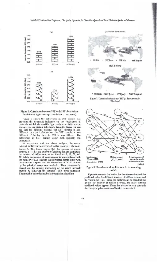
Figure 6. Correlation between SST.with SST observations for different lag (a: average correlation, b: maximum) Figure 7 shows•.the differences in SST domain that provides the dominant influence on the observation at particular rainfall stations (the figure only presents for station Sumurwatu and station Cikedung). From the figure we can see that for different stations, the SST domain is also different. In a particular station, the SST domain is also different, if the lag time for SST is also different. The differences in SST domain occur both spatially and temporally.

In accordance with the above analysis, the neural network architecture constructed in this research is shown in Figure 8. The figure shows that the number of output neurons is 13, i.e. the number of stations that are consistent, the number of hidden neurons are tested are 5, 10, 20, and 40. While the number of input neurons is in accordance with the number of SST clusters that correlated significantly with observations coupled with the dimension of GCM resulted by the principal component analysis. Then subsequently carried out the training and testing0f the neural network models by following the scenario 8-fold cross validation. The model is trained using back propagation algorithm.

(a)Station Sumurwatu

(b)Cikedtmg

[image:5.607.43.551.0.850.2]

• StanQn 'SST

June •

SS1'July "SST August

Figure 7. Domain di$ttibuticon()fSST (a; Sunmr",.;ltu; b:

Cikedung]

l>1PUt rewon: [Chlstered SST,

dimensmuess GeM]

Outputnruron :13

[image:5.607.312.536.34.571.2]

(accordanoe with numbera:>nsistl!l1Ol! statim)

Figure 8. Neural network architecture for downscaling models

HWlennewon:

5, 10,:;n,and. 40

(6)

*

•

I

zyxwvutsrqponmlkjihgfedcbaZYXWVUTSRQPONMLKJIHGFEDCBA

[image:6.595.58.552.14.826.2]

,

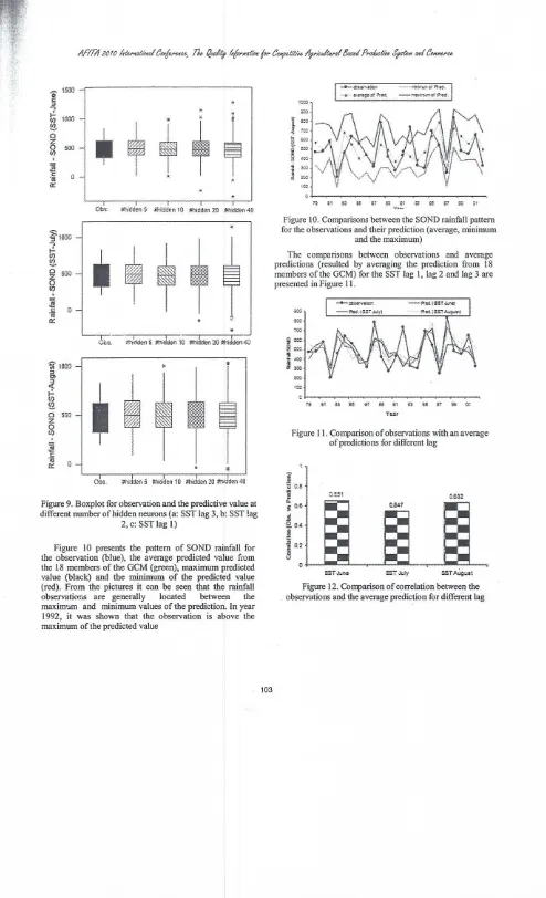
Figure 9. Boxplot for observation and the predictive value at different number of hidden neurons (a: SST lag 3, b: SST lag

2, c: SST lag I)

Figure 10 presents the pattern of SOND rainfall for the observation (blue), the average predicted value from the 18 members of the GCM (green), maximum predicted value (black) and the minimum of the predicted value (red). From the pictures it can be seen that the rainfall observations are generally located between the maximum and minimum values of the prediction. In year 1992, it was shown that the observation is above the maximum of the predicted value

1z:-t;

~~

l

ecc

~

1C~

~

5>X

i

~:t .)l ..:0::

l

?:D

zec

100

Figure 10. Comparisons between the SOND rainfall pattern for the observations and their prediction (average, minimum

and the maximum)

The comparisons between observations and average predictions (resulted by averaging the prediction from 18 members of the GCM) for the SST lag I, lag 2 and lag 3 are presented in Figure 11.

i ~-:~

ii1.w,

-!~ i'

L;"

zyxwvutsrqponmlkjihgfedcbaZYXWVUTSRQPONMLKJIHGFEDCBA

n m a ~ • a M a • • ~ ~

y"",

Figure II. Comparison of observations with an average of predictions for different lag

[image:6.595.54.292.42.495.2]

(7)

As presented in the Figure II, it can be seen that the overall pattern according to the pattern predicted observation. An extreme deviation occurred in 1988 and 1992. In 1987 up to 1995 shows that the downscaling technique is not able to follow the extremes pattern that exist in the data. Correlation between observations and predictions range from 0.547 to 0.651 as shown in Figure 12.

Figure 13 presents the scattered plots between observations and predictions. The figure demonstrates that for small values of observations, the predicted value tend to overestimate, and for the higher value of the observation that there tends to be underestimated.

1000

zyxwvutsrqponmlkjihgfedcbaZYXWVUTSRQPONMLKJIHGFEDCBA

"ib

~

."zyxwvutsrqponmlkjihgfedcbaZYXWVUTSRQPONMLKJIHGFEDCBA8 ) 0

l:

•

_1i

"

0>

~

8 ) 0

I-fIl

~"

.~

4 0 0

ti

'e

~

2tHl

20.0 400" 8 ) 0 1000

Observation

Figure 13. Scattered plot of the observation vs. prediction V. CONCLUSSION

Based on the experiment, we can conclude several things:

a. SST domain influencing the observations at a particular station varies temporally and spatially. In this case, different stations have different SST domain. At a station, if the lag is different, the domain in SST is also different.

b. SST with a lag (SST in August) gave the highest correlation with the observed data that is equal to 0.796. While the correlations for the lag 2 and lag 3 are 0.718 and 0.763, respectively.

c. ANN with hidden neuron 5 is capable for predicting SOND rainfall with correlation between observations and predictions, i.e. 0.651, 0.547, and 0.632 for the SST lag 3, lag 2 and lag I, respectively.

d. There is a tendency that the models overestimate low SOND rainfall and underestimate high SOND rainfall

found in the observed data.

zyxwvutsrqponmlkjihgfedcbaZYXWVUTSRQPONMLKJIHGFEDCBA

ACKNOWLEDGMENT

This research is part of Bogor Agricultural University's 1M-HERE B2c Project, which is funded by the National Government under contract number:

7/13.24.4/S P P /I- MHEREl2010. The authors thank to International Research Institute (IRI), Columbia University

for their permission to access the GCM datasets and to BMKG for providing the rainfall data.

REFERENCES

[IJ Wilby, R.L. and T.M.L. Wigly. Downscaling General CirculationModel Output : a Review of Methods and Limitations. Progressin PhisicalGeography21,4, pp. 530-"548,1997.

[2J Wigena, A.H. Pemodelan Statistical Downscaling dengan Regresi Projection Pursuit untuk Peramalan Curah Hujan Bulanan : KasusCurah Hujan Bulanan di lndramayu. PhD

Dissertation, Department of Statistics, Graduate School, Bogor AgricultureUniversity,Bogor2006.

[3J Sutikno. StatisticalDownscalingLuaran GCM dan Pemanfaatannya untuk Peramalan Produksi Padi. PhD Dissertation, Department

of Meteorology, Graduate School, Bogor Agriculture University, Bogor.2008.

[4J Boer, R. Metode untuk mengevaluasi Keandalan model Prakiraan Musim. Climatogylaboratory,Departementof Meteorology,Facultu

of Mathematics and Natural Sciences. Boger Agriculture University

Bogar.2006.