MODELLING AND SIMULATING
SPATIAL DISTRIBUTION PATTERN OF URBAN
GROWTH USING INTEGRATION OF GIS AND
CELLULAR AUTOMATA
(Case Study in Bandung Area
–
West Java Province)
ERWIN HERMAWAN
GRADUATE SCHOOL
BOGOR AGRICULTURAL UNIVERSITY
BOGOR
STATEMENT
I, Erwin Hermawan hereby states that this thesis entitled:
MODELLING AND SIMULATING
SPATIAL DISTRIBUTION PATTERN OF URBAN GROWTH USING INTEGRATION OF GIS AND CELLULAR AUTOMATA (CASE STUDY IN BANDUNG AREA – WEST JAVA PROVINCE)
is a result of my own work under the supervision of advisory board during the
period of February 2009 until March 2011 and that it has not been published ever.
The content of this thesis has been examined by the advisory board and external
examiner.
Bogor, April 2011
Erwin Hermawan
ABSTRACT
ERWIN HERMAWAN (2011). Modelling and Simulating Spatial Distribution Pattern of Urban Growth using Integration of GIS and Cellular Automata (Case study in Bandung Area – West Java Province). Under the supervision of HARTRISARI HARDJOMIDJOJO and IDUNG RISDIYANTO.
This research has a purpose to study and develop a model that can representing and simulating spatial distribution pattern of urban growth in Bandung Area. Integration of Geographic Information System (GIS) and Cellular Automata (CA) modelling was implemented to develop Urban Growth Spatial Distribution Model (UGSDM) in Bandung Area. GIS with spatial analysis used to prepare and process necessary data that are later incorporated into CA-based model.
Two scenarios have been implemented to calibrate and validate the result from simulation model. In the first scenario, driving forces and constrained factors (slope > 15%, protected forest, open green space and water body) as an input in the model simulation. Whereas, the second scenario is the simulation model will be run without slope > 15 % as a constraints in model input. Khat Coefficient for first and Second
scenario in 1991 – 2000 simulation model is for about 76,80 % and 82,66 % respectively, whereas in 2000 – 2007 is for about 76,26 % and 79,27 % respectively. Base on the result, second scenario is the best to be applying in model simulation and can be used to predicting urban growth simulation. This scenario will be reduces the impact of the mismatched cells in simulation model and making the simulation accuracies more realistic to reflect the actual condition in the real world.
The result from urban development simulation in 2015 and 2030, shows that urban development in Bandung area will continue in two ways: one is through the in-filling of areas within the currently existing urban in Cimahi and Bandung City, and another is through expanding toward the southeast of the Bandung area.
ABSTRAK
ERWIN HERMAWAN (2011). Pemodelan dan Simulasi Pola Distribusi Spasial Pertumbuhan Perkotaan menggunakan integrasi SIG dan Cellular Automata [ Studi Kasus wilayah Bandung, Provinsi Jawa Barat] Di bawah bimbingan dari HARTRISARI HARDJOMIDJOJO dan IDUNG RISDIYANTO.
Penelitian ini bertujuan untuk mempelajari dan membangun sebuah model yang dapat merepresentasikan dan mensimulasikan pola distribusi spasial pertumbuhan perkotaan di wilayah Bandung. Integrasi dari Sistem Informasi Geografis (SIG) dan Pemodelan Cellular Automata di implementasikan untuk membangun Model Spasial Pertumbuhan Perkotaan di wilayah Bandung. Analisa SIG di gunakan untuk mempersiapkan dan memproses data yang di butuhkan untuk kemudian di integrasikan ke dalam sebuah model berbasiskan Cellular Automata.
Dua skenario telah di implementasikan untuk mengkalibrasi dan memvalidasi hasil dari model simulasi. Pada skenario pertama, faktor penggerak dan faktor pembatas (kemiringan lereng > 15%, hutan lindung, ruang terbuka hijau dan tubuh air) digunakan sebagai input dalam model simulasi. Sedangkan, skenario kedua adalah model simulasi yang di jalankan tanpa menggunakan kemiringan lereng sebagai input di dalam model. Koefisien Khat yang dihasilkan untuk skenario pertama
dan kedua secara berturut-turut adalah sebesar 76,26 % and 79,27 % . Berdasarkan hasil tersebut, skenario kedua memberikan hasil yang terbaik untuk di aplikasikan dalam model simulasi dan dapat digunakan dalam prediksi pertumbuhan perkotaan. Skenario ini mengurangi dampak ketidak-sesuaian cell pada model simulasi dan membuat akurasi model simulasi lebih realistik untuk menggambarkan keadaan sebenarnya di dunia nyata.
Hasil dari simulasi perkembangan perkotaan di tahun 2015 dan 2030 menunjukan bahwa perkembangan perkotaan di wilayah Bandung akan berlangsung dalam dua cara : pertama memenuhi dan berkembang sepanjang wilayah perkotaan yang telah telah terbangun di Cimahi dan kota Bandung dan perkembangan lainnya adalah berkembang ke arah wilayah Bandung bagian tenggara.
SUMMARY
ERWIN HERMAWAN (2011). Modelling and Simulating Spatial Distribution Pattern of Urban Growth using Integration of GIS and Cellular Automata (Case study in Bandung Area – West Java Province). Under the supervision of HARTRISARI HARDJOMIDJOJO and IDUNG RISDIYANTO.
This research has a purpose to study and develop a model that can representing and simulating spatial distribution pattern of urban growth in Bandung Area. Integration of GIS and Cellular automata modelling was used to develop the urban growth simulation model. GIS with spatial analysis used to prepare and process necessary data that are later incorporated into CA-based model.
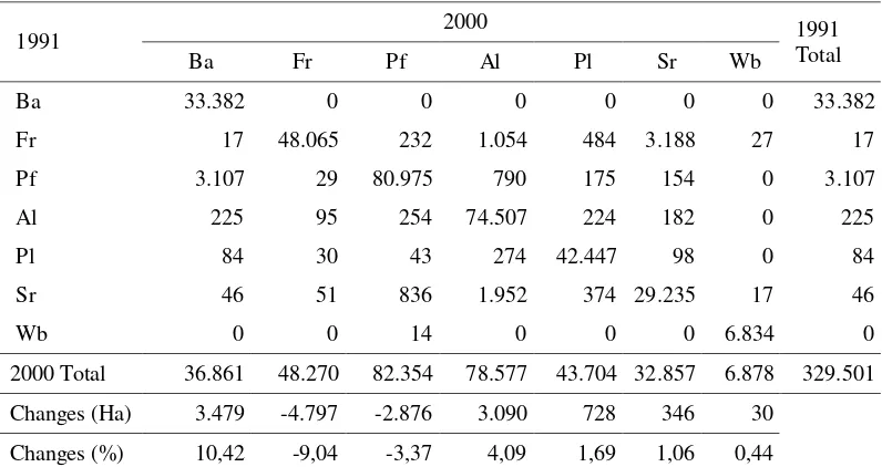
Analyze of markov chain change detection during 1991-2007 in Bandung area was done to analyze and detection trend probability conversion from Paddy field, Plantation, shrub and forest into built up-area. The result was shown that the largest increase of built-up area for each year development is the result from land conversion of paddy field into built-up area. Radial sprawl for built-up area development was impact to conversion from Paddy field to built-up area and make paddy field as the highest weighted for landcover priority conversion to built-up area.
Extraction driving forces and constraint information has been done using multi-criteria evaluation to derive weighted factors for urban development. Based on the result of weighted calculation, neighbourhood effect is the most important influence factors in built-up area development during 1991 – 2000 in study area. The weighted was contributing 48% for urban development. This condition was agreed with the theory, urban development usually takes place first in the adjacent area to the developed built-up area.
Furthermore, The analysis result from multicriteria evaluation of driving forces and determine of landuse conversion priority using markov change detection were used as an information and data input in system configuration and development of urban growth simulation model.
In this research, Integration of GIS and Cellular automata modelling was used to develop a simulation model that can represent spatial distribution pattern of urban growth in Bandung Area. CA can be considered as analytical engine of GIS, which plays in important role in modelling and simulation of spatial-temporal processes. Another approach to integrate CA and GIS in this research are to develop a standalone CA program that can use data from GIS. Data interchange and compatibility can be achieved through file conversion protocols.
All of the data are contained in a grid-like shape based vector polygon with the
spatial resolution of the cell in 100 x100 m. it’s means, each cell on the model
converted and standardized into spatial resolution for each cell 100 x 100 m. The second one is limitation of the computer specification to run and process the spatial database in the model simulation. Bandung as a study area , around of area is for about 329.510 Ha. This cell size was chosen to simplify in computing of the spatial database in the model processing.
Each cell in the database has unique coordinate system which describe in Cartesian coordinate. The same column in the lattice has the same of y-coordinates, the other way the same row has the same of x-coordinate. The attributes cell contains information of driving forces (Slope, Neighbourhood, distance from road and Urban Hierarchy Index), landcover priority and cell state in year –t (Urban existing, Urban allocation and constraint area).
Hybrid approach was implemented to integrate between tabular and spatial data as a Spatial Database Management System (SDBMS) in development of Urban Growth Spatial Distribution Model (UGSDM) in Bandung Area. In this study, UGSDM was developed to modelling and simulating spatial distribution of urban growth in Bandung area using integration of GIS and cellular automata methods.
Model calibration is the process of modifying the input parameters in an attempt to match field conditions within some acceptable criteria until the output from the model matches an observed set of data. In this study, two scenarios were applied to calibrate the model. In the first scenario, driving forces and constrained factors (slope > 15 %, protected forest, open green space and water body) as an input parameter in the model simulation. Whereas, the second scenario is the simulation model will be run without slope as an input parameter.
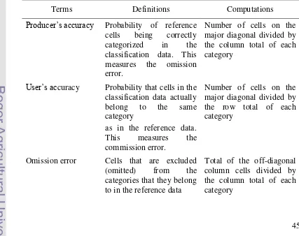
Meanwhile, Validation is the evaluation of the predicted modelling results. Simulation accuracy assessments were applied in model validation process. It can be defined as the task of comparing two maps: one generated by the model (data to be assessed), and the other based on the ground truth (the reference data). The reference data were assumed accurate and forms the standard for comparison. The error matrix approach and kappa analysis are methods in accuracy assessment that applied in this study.
In this research, Model simulation was running from 1991 – 2000 and 2000 – 2007 to calibrate and validate the model result. Khat Coefficient for first and Second
scenario in 1991 – 2000 simulation model is for about 76,80 % and 82,66 % respectively, whereas in 2000 – 2007 is for about 76,26 % and 79,27 % respectively. Base on the result, second scenario is the best to be applying in model simulation and can be used to predicting urban growth simulation. This scenario will be reduces the impact of the mismatched cells in simulation model and making the simulation accuracies more realistic to reflect the actual condition in the real world.
The result from urban development simulation in 2015 and 2030, shows that urban development in Bandung Area will continue in two ways: one is through the in-filling of areas within the currently existing urban in Cimahi and Bandung City, and another is through expanding toward the southeast of the areas.
Copyright @2011, Bogor Agricultural University Copyright are protected by law,
1. It is prohibited to cite all of part of this thesis without referring to and mentioning the source:
a. Citation only permitted for the sake of education, research, scientific writing, report writing, critical writing or reviewing scientific problem b. Citation does not inflict the name and honor of Bogor Agricultural
University
MODELLING AND SIMULATING
SPATIAL DISTRIBUTION PATTERN OF URBAN
GROWTH USING INTEGRATION OF GIS AND
CELLULAR AUTOMATA
(Case Study in Bandung Area
–
West Java Province)
ERWIN HERMAWAN
A Thesis submitted for the Degree of Master of Science in Information Technology for Natural Resources Management Program Study
GRADUATE SCHOOL
BOGOR AGRICULTURAL UNIVERSITY
BOGOR
Research Title : Modelling and Simulating Spatial Distribution Pattern of Urban Growth using Integration of GIS and Cellular Automata (Case study in Bandung Area – West Java Province)
Name : Erwin Hermawan
Student ID : G051060011
Study Program : Master of Science in Information Technology for Natural Resources Management
Approved by,
Advisory Board
Dr. Ir. Hartrisari Hardjomidjojo, DEA Supervisor
Idung Risdiyanto, S.Si, M.Sc Co-Supervisor
Endorsed by,
Program Coordinator
Dr. Ir. Hartrisari Hardjomidjojo, DEA
Dean of Graduate School
Dr. Ir. Dahrul Syah, M.Agr.Sc
Date of Examination : January 25, 2011
ACKNOWLEDGEMENTS
First of all, I would like to express my highest gratefulness to Allah SWT,
for His blessing, His will, His power, His help and His guidance to me during my
study.
I wish to show my gratitude to my supervisor Dr. Ir. Hartrisari
Hardjomodjojo, DEA. and my co-supervisor Idung Risdiyanto, S.Si, M.Sc. for
their patience, advices, guidance, valuable inputs, time, encouragement and
constructive criticism during the supervision of my research. and also I would like
to thank to Dr. Ibnu Sofyan, M.Eng., as the external examiner of this thesis for his
positives ideas and inputs.
I would like to thank to my kindly classmates MIT-NRM IPB batch 2006
for their friendliness, togetherness and best years in study time, and also to all
MIT students generally. I thanks also MIT secretariat and staff for their
cooperation and friendliness during study. Moreover, to all MIT lectures, I really
appreciate for their sharing of valuable knowledge and experiences. Highest
thanks is also addressed to my friend, Andri Susanto, S.Si to discuss about GIS
and Remote sensing actually in Spatial Database Programming.
My deep appreciation is extended to my family members ; my father H.
Mumuh Efendi, my Mother, Hj. A. Kurniasih and my sister Riska Rostikawati,
SE., for being a source of motivation, encouragement, love, cares, patience and
above all prayed for me during finishing my study in IPB.
Last but not least, my lovely “An-Nisa Larasati Budhiyono, ST.” thanks for your love, cares and support at the end of my research study.
CURRICULUM VITAE
Erwin Hermawan was born in Sumedang, West Java,
Indonesia, on January 26th 1982. He spent his childhood in Sumedang until study in senior High School at SMU 1
Cimalaka, Sumedang in 2000. He achieved his
undergraduate degree in 2005 from Bogor Agricultural
University, Faculty of Mathematics and Natural Science,
majoring in Meteorology.
In 2006, Erwin Hermawan pursued his Master Degree at Master of Science
in Information Technology for Natural Resource Management (MSc in IT for
NRM) Master Degree program of Bogor Agricultural University. His final project
for thesis is entitled “ Modelling And Simulating Spatial Distribution Pattern of Urban Growth using Integration of GIS And Cellular Automata (Case Study in
i
CONTENTS
Page
CONTENTS………. i
LIST OF TABLES……… iv
LIST OF FIGURES……….. v
LIST OF APPENDICES……….……….. vii
I. Introduction………...……… 1
1.1. Background……….. 2
1.2. Research Objective………...………… 2
1.2.1. Main Objectives………... 2
1.2.2. Specific Objectives………...……… 2
1.3. Scope, Limitation and Assumption of Research………..…… 3
1.4. Time and Study Area of Research……….……….…. 3
1.5. General of Research Methodology………..………. 4
1.6. Thesis Output………...……… 7
1.7. Thesis Structure………..…….. 7
II. Analysis of Markov Chain Change Detection and Driving Forces of Urban Growth Development in Bandung Area during 1991 – 2007……. 9
2.1. Introduction……….. 9
2.1.1. Background……….…. 9
2.1.2. Objective………..… 9
2.2. Literature Review ………...…. 9
2.2.1. Urban Growth and Urban Sprawl……….…… 9
ii
2.2.3. Markov Change Detection……… 13
2.2.4. Multi-criteria Evaluation for Built-up Area Suitability…… 14
2.3. Methodology……….. 15
2.3.1. Preparation and Processing of Necessary Data……… 15
2.3.2. Priority of Landcover conversion using Markov Change Detection……….. 16
2.3.3. Calculation of Driving Forces……….. 19
2.3.4. Multi-criteria Evaluation of Driving forces……….. 22
2.4. Result and Discussion……….……….……… 25
2.4.1. Data Preparation and Processing of Driving Forces ……... 25
2.4.2. Weighting Factors calculation of Driving Forces……….. 28
2.4.3. Change detection in Bandung Area………. 29
2.4.4. Transitional Matrix and Weighted Factors of Landcover Priority ……….…… 33
2.5. Conclusion………..………… 38
III. Development of Urban Growth Simulation Model Using Integration of GIS and Cellular Automata ……….……. 39
3.1. Introduction……….. 39
3.1.1. Background……….…. 39
3.1.2. Objective………..… 39
3.2. Literature Review ………...…. 40
3.2.1. The Concept of Cellular Automata……….. 40
3.2.2. CA in Urban Modelling ……….……….. 40
3.2.3. Integrating GIS and CA for Urban Dynamics Modelling… 43
3.2.4. Model Calibration and Validation ………...…… 44
3.3. Methodology……….... 46
3.3.1. Database and Model Development ……….……... 46
iii 3.3.3. Population Projection ……….………. 50
3.3.4. Relation between Amount of Population and Built-up Area ………. 50
3.3.5. Configuration of Model, Calibration and Validation ….… 51
3.4. Result and Discussion……….……….……… 52
3.4.1. Configuration of Model Structure and Element………...… 52
3.4.2. Population Projection and Land Demand for Built-up Area 55
3.4.3. Logical Framework and Program Flow ………….………. 57
3.4.4. Calibration and Validation Model using Two Scenarios … 60
3.4.5. Projection of Urban Growth Spatial Distribution Model… 64
3.4.6. Urban Land Carrying Capacity in Bandung Area………… 66
3.5. Conclusion………..………… 67
IV. General Conclusions and Recommendations
4.1. Conclusions………... 69
4.2. Recommendation……….. 70
iv
LIST OF TABLES
Page
2.1 Raster Data……….. 15
2.2 Vector Data………. 15
2.3 Non-Spatial Data……….……… 16
2.4 List of Software………..………. 16
2.5 Driving forces and Constraints Regulation for Urban Development….. 19
2.6 UHI Processing………..………. 21
2.7 Weighted for Driving Forces using Ranking Methods………..………. 28
2.8 Landcover Classification Type in study area……….………. 29
2.9 Landcover Change in Study Area during 1991 – 2007……...………… 32
2.10 Percentage of Landcover Change in Study Area during 1991 – 2007… 32 2.11 Landcover Change Transitional Matrix, 1991– 2000 (in hectares)….... 34
2.12 Landcover Change Transitional Matrix, 2000 – 2007 (in hectares)…... 35
2.13 Landcover Transitional Probabilities, 1991–2000………….…………. 36
2.14 Landcover Transitional Probabilities, 2000 – 2007……… 36
2.15 Probability Trend Conversion from each Landcover Type to Built-up Area during 1991 – 2007………. 37
2.16 Weighted for each Landcover type………...……….. 37
3.1 Definitions of Terms in an Error Matrix and Their Computations….… 45
3.2 List of Software………..………. 47
3.3 Data Input to Predict Land Demand for Settlement Area……..………. 55
3.4 Built-up Area,Population and Density in 1991, 1997, 2000 and 2007... 56
3.5 First Scenario Simulation Result………. 62
3.6 Second Scenario Simulation Result……….. 63
3.7 Urban Development base on suitability of Slope Range….……..…… 63
3.8 Khat Coefficient for Two Scenarios... 64
v
LIST OF FIGURES
Page
1.1 Research of Study Area.……….……….……… 4
1.2 General Methodology of Research………..……… 6
2.1 Forms of Sprawl………..….. 11
2.2 Priority of Conversion using Markov Change Detection………...……. 18
2.3 Calculating of Road Network Effect……….….. 22
2.4 The Expected Relation between Slope and Urban Land………….…… 22
2.5 Slope Derivation from DEM………..……. 23
2.6 The Multi-criteria Evaluation Process……….……… 23
2.7 Neighbourhood Effect………...….. 25
2.8 Road Network effect………..……. 26
2.9 Slope Effect……….……… 26
2.10 Urban Hierarchy Index……….... 27
2.11 Constraints Area……….. 27
2.12 Landcover Type Classification in Bandung Area, 1991………. 30
2.13 Landcover Type Classification in Bandung Area, 1997………. 30
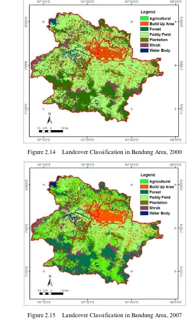
2.14 Landcover Type Classification in Bandung Area, 2000………. 31
2.15 Landcover Type Classification in Bandung Area, 2007………. 31
2.16 Landcover Type Areas in 1991, 1997, 2000 and 2007………... 33
3.1 Two dimensional Cellular Automata (Torrens,2000)………... 42
3.2 Database Schematic………. 46
3.3 Hybrid Approach to build GIS Application Software ………. 47
3.4 Schematic Diagram of the Proposed………... 49
3.5 Regression and Correlation Analysis to get Demand for Prediction Model…. 50
3.6 Model Calibration and Validation Process……….. 51
vi 3.8 Lattice and Cells Attributes………...….. 54
3.9 Relation between The Increase of Population and Built-up Area……. 56
3.10 Logical Framework of Model Development between…………..……. 57
3.11 A flowchart Showing The Simulation of The Model……… 59
3.12 Urban Development in 1991 – 2000 using 1st Scenario….…………. 60
3.13 Urban Development in 2000 – 2007 using 1st Scenario……..……… 61
3.14 Urban Development in 1991 – 2000 using 2nd Scenario…….……… 61
3.15 Urban Development in 2000 – 2007 using 2nd Scenario…….……… 62
3.16 Urban Development Simulation in Bandung Area, 2015……… 65
3.17 Urban Development Simulation in Bandung Area, 2030……… 65
vii
LIST OF APPENDICES
Page
1 Performance of UGSDM Application.……….…………... 75
1
I.
INTRODUCTION
1.1. Background
Urban development and the migration of the population from rural to urban
areas are considered as significant global phenomena. This has attracted a lot of
attention to the study of urban development under the theme of global
environmental change (Liu, 2009). Through a better understanding of the
mechanism of urban development process, the urban planner and manager could
be reduce the risk of wrong or bad decisions and enhance the effectiveness of new
plans. Various urban models have been built a model to get a better understanding
of the urban expansion phenomena.
In order to be useful and realistic, urban models depend on real world data
that can be integrated and mapped in a modelling scenario. Existing urban land
uses and growth patterns, existing road network, location of various facilities,
availability and infrastructure facilities are the example of the data can be used in
urban modelling scenario. Geographic Information Systems (GIS) has emerged as
a prime framework for the integration and management of a range of spatial real
world data. However, to use GIS alone as modelling tool have been received with
skepticism as it has limited modelling functionalities and has constraints in
handling temporal data sets. Furthermore, modelling and simulations in the spatial
domain extensively have done using the techniques of Cellular Automata (CA),
although there are different approaches to model processes in space and time
including the geostatistical approaches. Cellular Automata (CA) plays in
important role in modelling and simulation of spatial-temporal processes.
Nevertheless, GIS and CA in combination can be used as a strong couple to
model the urban growth to take advantages of both the techniques. In case of GIS,
its spatial data analysis capacities may be insufficient to handle complex urban
dynamics. The integration of the dynamic strength of CA with the effective spatial
representation found in GIS thus may be beneficial to achieve realistic
2 In this research, a simulation model to study and prediction the spatial
distribution pattern of urban growth in Bandung Area was developed by using
integration of CA and GIS modelling. CA can be considered as analytical engine
of GIS, which plays in important role in modelling and simulation of
spatial-temporal processes. Another approach to integrate CA and GIS in this research are
to develop a standalone CA program that can use data from GIS. Data interchange
and compatibility can be achieved through file conversion protocols.
Bandung area including Bandung Municipality, Bandung Regency, Cimahi
Municipality and West Bandung Regency were selected as study area in this
research. Bandung is capital city of west java province and one of metropolitan
city in Indonesia, which has a very density population in the city center. The new
constructions mainly taken place in the fringe urban areas of Bandung area. In this
research, urban growth driving forces as a factor influences in urban development
was defined and translated into the model structure to regulate the Urban CA
model. Some scenario defining CA rules was generated to calibrate and validate
the simulation model. The best simulation scenario will be used and applied to
simulating and predicting spatial distribution pattern of urban growth in Bandung
area in the future years.
1.2. Research Objective
1.2.1.Main Objective
This research has a purpose to study and develop a model that can represent
spatial distribution pattern of urban growth in Bandung Area. Integration of GIS
and Cellular automata modelling was used to develop the urban growth simulation
model.
1.2.2.Specific Objective
The specific objectives of this research are:
1) To define and analyze driving forces of urban growth and landcover priority
conversion using markov chain change detection in Bandung Area during
3 2) To develop model capable of representing spatial distribution pattern of
urban growth in Bandung area using integration of GIS and Cellular
Automata Modelling.
3) To generate alternative scenario was implemented in urban CA simulation
model.
1.3. Scope, Limitation and Assumption of Research
Scope, limitation and assumption of this research are:
1) Study area as a boundary of system in this research is Bandung area,
including : Bandung Municipality, Bandung Regency, Cimahi Municipality
and West Bandung Regency
2) Integration of GIS and Cellular Automata was applied to achieve the goal
from this research.
3) In the realiality of urban development, natural hazard can be added as a
constrain factor. In this research natural hazard didn’t included in modeling of urban growth. Slope effect can be assumed as a factor related to natural
hazard assessment.
1.4. Time and Study Area of Research
This research was conducted from August 2009 until December 2010, including
data preparation, data processing and make a final report in MIT Laboratory, Bogor -
West Java. Meanwhile, data collecting was taken in Bandung – West java.
The study area is Bandung Area which located in region of West Java Province.
Recently, Bandung Area can be divided into four regions, there are Bandung
Municipality, Bandung Regency, Cimahi Municipality and West Bandung Regency as
shown in Figure 1.1. Geographically, it is located between 107022’– 1080,53’ east longitude and 60,41’– 70,19’ east longitude.
Topographically, The highland point area in the north is 1.050 m and the lowland
in the south, which elevation 675 m above sea level. The land in South Bandung until the
line of grade crossing. The land is relatively flat, meanwhile the north part is mountainous
where one could see Bandung shape and gaze at the whole city panorama. Geological
4 mount explosion. The kind of materials in the north generally andosol in the south and
east consist of greey alluvial with clay sediment while in central and west scattered
andosol.
Figure 1.1 Research of Study Area.
The climate of Bandung mostly influenced by the mountains, so that the
weather is humid and cool. Nowadays, a change to weather occurs. The
temperature average extremely rose, which in October 2009 the temperature reach
out 31, 6 0C. That phenomena mainly caused by air pollution from motor cycle and global heat. Even that so, the average of rainfall frequency is still high.
1.5. General of Research Methodology
General of research methodology for Modelling Spatial Distribution Pattern
of Urban Growth using Cellular Automata in Bandung area, can be seen in Figure
5 data. Spatial data can be divided into raster and vector data. Topographical maps
(Rupa Bumi Indonesia) which covering Bandung area was used as vector data, including layers of Administrative boundary, landuse and Road Network.
Meanwhile, satellite imagery including SRTM-DEM, SPOT 5 and Landsat TM
imagery were used as a raster data in this research. Statistical data, including time
series of population and village potential statistics of Bandung area in 1991, 1997,
2000 and 2007 was used as non-spatial data to predict population projection.
Data processing using various statistics methods and spatial analysis
technique in GIS have been applied to derive the data input into the development
model. On the other hand, landcover type classification was get from references
map and derive from satellite imagery in 1991, 1997, 2000 and 2007. Markov
chain change detection was applied to analyze trend of change detection during
the periode 1991 – 2007 in Bandung area. The result from this analysis is trend of landcover priority conversion into built-up area. Furthermore, land demand for
up area was derived from relation between population projection and
built-up area in the same years.
Driving forces and constraints, which are influence for urban development
was derived based on regulation from study literature. Standardization value for
each driving forces and constrain into 0 – 1, and then Multicriteria evaluation as a transition rule was applied to get weighted from each driving forces and there
contributes for urban development. Landcover priority that’s means priority for
each type of landcover conversion into built up area was combine with potential
value which derive from driving forces and constraints.
Furthermore, land demand for built-up area was related into ranking of
potential value. In this step, the model will be indicated that the number of the
cells who have higher potential values will be translated into built-up area
development base on amount of land demand requirement for built-up area in year
- t+n. Model calibration and validation using some scenario was applied to calculate simulation accuracies of the urban growth spatial distribution model. The
best scenario from the result will be applied in model simulation and can be used to
6 Driving Factors
Neighbourhood Effect Road Network Urban Hierarchy Index Slope 0 – 15 %
Constraints Factors
Slope > 15 %
Forest Protected, Green Space Area, Water Body
Standardization Factors Landcover
Classification in 1991, 1997, 2000 and 2007 from Satellite Imagery
Markov Chain Change Detection Population
Data in 1991, 1997, 2000 and
2007
Built-up Area in 1991, 1997, 2001
and 2007
Projection Population in year t+n
Land Demand of Built-up Area in Year t+n Relation between
Population and Built-up Area
Weighted using Ranking Methods
Multicriteria Evaluation to get Potential Cell
Transition Potential Value
Ranking of Potential Value
Allocate Potential Value into Built-up Area in Year t+n
Conversion priorities of each landcover type into
Built-up area
Calibration & Validation Model with Actual Built Up Area in
year t+n
Future Spatial Distribution of Urban Growth Simulation in Bandung Area Yes
No Reference of
Landuse landcover map in 2000 and
2007
7 1.6. Thesis Output
Several output of this research are:
1) A model simulation to support decision related to projection population and
to know spatial distribution pattern of urban growth in Bandung area.
2) Alternative maps based on scenario created to predict spatial distribution of
built-up area.
1.7. Thesis Structure
The thesis was organized into three chapters. The first chapter describes
introduction chapter includes: (1) Background, (2) Research objective (3) Scope .
limitation and assumption of research (4) Time and study area of research, (5)
General of Research Methodology, (6) Thesis Output and (7) Structure of Thesis
document.
Generally, the result and analyze from this research activity are described in
chapter 2 and chapter 3. In the second chapter, analysis of markov chain change
detection and driving forces of urban growth in Bandung area was analyzed and
discussed. Data processing using various statistics methods and spatial analysis
technique in GIS have been applied to derive the data input into the development
model. Population projection and it’s relation with demand of built-up area, multicriteria evaluation of driving forces and determine of landuse conversion
priority using markov change detection were applied in this data processing and
was used as an information and data input in system configuration and
development of urban growth simulation model.
The Third chapter describes development of urban growth simulation
model, calibration and validation of the model. In this research, two scenarios
were applied in urban growth cellular automata simulation model to calibrate the
model. Validation using accuracy assessments with error matrix and kappa
coefficient were applied to validate the best of scenario result. Finally, general
conclusion and recommendation are drawn in fourth chapter as last chapter of this
9
II.
ANALYSIS OF MARKOV CHANGE DETECTION AND
DRIVING FORCES OF URBAN GROWTH
DEVELOPMENT IN BANDUNG AREA
DURING 1991 - 2007
2.1. Introduction
2.1.1.Background
Driving forces and constrains are the keys factors in the urban growth
development context. Driving forces can be defined as causes or factors influence
for urban growth modeling. In this research, slope, road network, Neighbourhood
effect and Urban Hierarchy Index were selected as a driving forces input in
modeling of urban growth development in Bandung Area. Whereas, protected
forest, slope greater than 15% , open green space and water body were selected as
a constraints factor in this study area.
Furthermore, trend of priority conversion between each landcover type into
built-up area during 1991 – 2007 in Bandung area was analyzed using markov chain change detection technique. The analysis result from this processing were
used as an information and data input in system configuration and development of
urban growth simulation model.
2.1.2.Objective
The objectives of this study is to define and analyze driving forces of urban
growth and landcover priority conversion using markov chain change detection in
Bandung Area during 1991 - 2007.
2.2. Literature Review
2.2.1.Urban Growth and Urban Sprawl
Urban growth indicates a transformation of the vacant land or natural
environment to the construction of urban fabrics including residential, industrial
and infrastructure development, it mostly happened in the fringe urban areas.
10 (Shenghe and Sylvia, 2002). It has always been the focus of the social economic
debates due to its impacts on social economic aspects as well as the impacts on the
huge consumption of cultivated lands and damage to the environmental
sustainability.
Urban sprawl, also known as suburban sprawl, is the spreading of a city and
its suburbs over rural land at the fringe of an urban area. Sprawl generally infers
to the increase in built-up and paved area with impacts such as loss of agricultural
land, open space, and ecologically sensitive habitats. Also, sometimes sprawl is
equated with growth of town or city (radial spread). In simpler words, as
population increases in an area or a city, the boundary of the city expands to
accommodate the growth; this expansion is considered as sprawl. Sprawl also
takes place on the urban fringe or the peri-urban region, at the edge of an urban
area or along the highways (Sudhira et al., 2004a).
Sprawl development consists of three basic spatial forms: low-density
(radial) sprawl, ribbon and leapfrog development (Barnes et al., 2001). Radial
sprawl is the consumptive use of land for urban purposes along the margins of
existing areas. This type of sprawl was supported by piece meal extensions of
basic urban infrastructures such as water, sewer, power, and roads. Ribbon sprawl
is development that follows major transportation corridors outward from urban
cores. In this case, lands adjacent to corridors are developed, but those without
direct access remain in rural uses/covers. Over time these nearby “raw” lands
maybe be converted to urban uses as land values increase and infrastructure is
extended perpendicularly from the major roads and lines. The leapfrog
development is a discontinuous pattern of urbanization, with patches of developed
lands that are widely separated from each other and from the boundaries, albeit
blurred in cases, of recognized urbanized areas (Barnes et al., 2001). This form of development is the most costly with respect to providing urban services such as
11 Radial Sprawl Ribbon Sprawl Leapfrog Sprawl
Figure 2.1 Form of Sprawl
In industrialized countries the future growth of urban populations will be
comparatively modest since their population growth rates are low and over 80%
of their population already live in urban areas. Conversely, developing countries
are in the middle of the transition process, when growth rates are highest. The
exceptional growth of many urban agglomerations in many developing countries
is the result of a threefold structural change process: the transition away from
agricultural employment, high overall population growth, and increasing
urbanization rates (Grubler, 1994).
Mapping and quantification of urban sprawl provides a picture of location of
sprawl, type and patterns of sprawl, which helps to identify the environmental and
natural resources threatened by such sprawls. Analysing the sprawl over a period
of time will help in understanding the nature and growth of this phenomenon and
thereby visualizing the likely scenarios of future sprawl (Sudhira et al., 2004a).
2.2.2.Urban Growth Driving Forces and Constraints
Urban growth driving forces can be simply defined as causes or factors
influence for urban growth modeling and in the opposite, whereas constraints are
limitations imposed by nature or by human beings that do not permit certain
action to be taken (Keeney, 1980). Definition for each driving forces and
12 1) Driving forces
a) Neighbourhood effect
Urban form itself has a very heavy influence on the urban
development. At a small scale, a city tends to grow in the areas
nearby the developed urban area. Neighborhood (the total number of
developed cells), in another word, the transition from non-urban to
urban was much affected by the adjacent area. If the vicinity of a cell
is developed area, this cell has much higher potential to transit to
urban form if it was non-urban before.
b) Road network
Road network have proved to be the key factor in urban evolution
process. It heavily impacts the urban form and land price and even the
location of city center and sub-center. While the relationship between
road network and urban form is far from clear. Closer the distances
from the city centre and the roads, the land has higher probability of
becoming developed.
c) Urban Hierarchy Index
An urban hierarchy categorizes centers according to their importance
in terms of the functions that they provide. Functional importance is
reflected in the range and amount of services and facilities. There is
usually (but not always) related to the size of the urban population.
Scalogram or Gultman Scaling is one of methods to ranks cities and
municipalities in a region by their functional complexity based on the
number and types of facilities that are located within them (Rustandi,
2008). The uses of the scalogram are to:
Categorize settlements into levels of functional complexity, Determine the types and diversity of services and facilities,
Indicate the sequence in which settlements tend to accumulate
13 Show the degree of access that people have to services and
facilities, and
Assist in deciding appropriate investment for settlements on a
hierarchical basis.
d) Slope effect
Ordinarily, built-up area will grow where there are flatten areas. The first
assumption of this method is that some areas are not developed because they
are too steep. The second assumption is that increasing slope implies a
higher building cost. With this assumption follow, that there should be a
lower percentage of cells within higher slope intervals, compared to lower
slope intervals. In this case, slope will constrain the urban form mainly
depends on the slope.
2) Constrained factors:
Constraints are limitations imposed by nature or by human beings that do
not permit certain action to be taken (Keeney, 1980). The specification of
constraint is typically based on available resources and regulations and involves
value or professional judgment.
The constrained factors indicate those limitations posed on the urban
devel-opment such as water body is not allowed to develop into urban use, high slope
terrain is not suitable for urban use, reserved area and public green area is not
allowed to transfer into urban, etc.
2.2.3.Markov Changes Detection
Landuse and landcover changes are the result of the complex interaction
between human and biophysical driving forces that act over wide range of
temporal and spatial scale. Change detection is a task to compare two sets of
imagery to identify changes of Landuse and landcover. The use of satellite data
enables change detection to be done over broad spatial scales. Markov chains have
been used to model changes in land use and land cover at a variety of spatial
scales. This type of change detection technique is one application of change
detection that can be used to predict future changes based on the rates of past
14 Land use studies using Markov chain models tend to focus on a much larger
spatial scale, and involve both urban and non-urban covers (Drewett, 1969;
Bourne, 1971; Bell, 1974; Bell and Hinojosa, 1977; Robinson, 1978; Jahan, 1986;
Muller and Middleton, 1994). The method is based on probability that a given
piece of land will change from one mutually exclusive state to another (Aavikson
1995). These probabilities are generated from past changes and then applied to
predict future change. Brown et al. (2000) recently presented an approach to estimating transition probabilities between two binary images in a study of land
use and land cover relationship in the Upper Midwest, USA. This approach,
according to Huber (2001), needs to be improved and generalized in order to
estimate properly Markov transitions from a pair of images.
The use of satellite imagery would create an opportunity for improved
analysis. Moreover, the Markov models have been mostly employed for studies
around a city or a slightly larger area, with a regional concentration in North
America. The application of stochastic models to simulate dynamic systems such
as land use and land cover changes in a developing nation is rare. Clearly, much
work needs to be done in order to develop an operational procedure that integrates
the techniques of satellite remote sensing, GIS, and Markov modelling for
monitoring and modelling land use and land cover changes.
2.2.4.Multi-criteria Evaluation for Built-up Area Suitability.
White et al., (1997) suggest the utility of assigning suitability of any cell for being allocated into built-up in the CA transitional rules. This concept has also been
subsequently applied in various other CA models (Singh, 2003; Sun, 2003).
Multi-criteria evaluation (MCE) is a method for combining many layers or Multi-criteria. A
criterion can be a factor or a constraint (Eastman, 1999). On the similar lines, the
multi-criteria evaluation was carried out for evaluating suitability of land cover to be
allocated into built-up. The availability of suitable land is another prime factor for
urban sprawl. The chief land use / land cover classification carried out for the satellite
imagery includes, already developed (built-up) area, water bodies (sea, rivers,
streams, tanks, lakes, etc), area under vegetation (agriculture, plantation, paddy, etc)
15 already developed areas and water bodies act as constraints for any further
development. However, the probability of open land, barren land and uncultivated
land for future built-up is very high. Similarly, the possibility of area under vegetation
to be converted into built-up as a result of sprawl cannot be ruled out.
2.3. Methodology
2.3.1.Preparation and Processing of Necessary Data
Several spatial and non-spatial data were prepared and used to defined and
analyze driving forces of urban growth and landcover priority conversion using
markov chain change detection in Bandung Area during 1991 – 2007. Spatial data consist of raster and vector data can be listed in Table 2.1 and 2.2. Meanwhile, non
-spatial data requirement can be seen in Table 2.3.
Table 2.1 Raster Data
No Data Coverage Aquitition Date Spatial Resolution
Source of The Data 1. Landsat 5
TM
Path/Row : 121/065 & 122/065
July, 5th and 28th 1991 Oct,15th and
22th 1997
30 m LAPAN 1)
2. SPOT 5 KKK/JJJ : 285/364 & 287/364
July, 17th 2007 20 m LAPAN 1)
3. DEM SRTM_f03_ s008e112
2000 90 m SRTM 2)
1) National Institute of Aeronautics and Space (Lembaga Penerbangan dan Antariksa Nasional) 2) Shuttle Radar Topographic Mission (SRTM). Can be free downloaded from the internet at
ftp://ftp.glcf.umiacs.umd.edu/glcf/landsat/WRS2/.
Table 2.2 Vector Data
No Data Type Date
Production Scale Source of The Data 1. Topographical
Map (Rupa Bumi Indonesia)
2000 1 : 25.0000
BAKOSURTANAL1)
2. Landuse Map 2000 & 2007 1 : 50.0000
BPN Bandung2)
1) National Coordinator for Survey and Mapping Agency ( Badan Koordinasi Survei dan Pemetaan Nasional)
16 Table 2.3 Non-Spatial Data
Data Type Date Production Source of Data
Population Data 1991 - 2008 BPS1) Village potential statistics (Potensi
Desa) 1991 and 2000 BPS
1)
1) Central Statistics Agency (Badan Pusat Statistik)
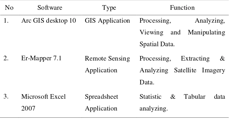
Several software were used to process the necessary data consist of Microsoft
Office, GIS and Remote Sensing application software. The following application
[image:34.595.113.511.322.531.2]software can be seen in Table 2.4.
Table 2.4 List of Software Application
No Software Type Function
1. Arc GIS desktop 10 GIS Application Processing, Analyzing,
Viewing and Manipulating
Spatial Data.
2. Er-Mapper 7.1 Remote Sensing
Application
Processing, Extracting &
Analyzing Satellite Imagery
Data.
3. Microsoft Excel
2007
Spreadsheet
Application
Statistic & Tabular data
analyzing.
2.3.2.Priority of Landcover Conversion using Markov Change Detection.
Markov Chain change detection is one application of change detection that
can be used to predict future changes based on the rates of past change, based on
probability that a given piece of land will change from one mutually exclusive
state to another.
Markov chain models have several assumptions (Parzen, 1962; Haan, 1977;
Wang, 1986; Stewart, 1994). One basic assumption is to regard land use and land
cover change as a stochastic process, and different categories are the states of a
17 of the process at time t, Xt, depends only on its value at time t-1, Xt-1,and not on
the sequence of values Xt-2, Xt-3,...,X0 that the process passed through in arriving at
Xt-1.It can be expressed as:
0 0 1 1 1
1
| , ,...,
|
t j t i
t j t i
P X a X a X a X a P X a X a
(1.1)
Moreover, it is convenient to regard the change process as one which is
discrete in time (t = 0,1,2,...). The P X
t aj|Xt1 ai
, known as the one-step transitional probability, gives the probability that the process makes the transitionfrom state ai to state aj in one time period. When steps are needed to implement
this transition, the P X
t aj |Xt1ai
is then called the step transition probability, Pij( ). If the( )
ij
P is independent of times and dependent only upon
states ai, aj and , then the Markov chain is said to be homogeneous. The
treatment of Markov chains in this study will be limited to first order
homogeneous Markov chains. In this event:
P X
t aj|Xt1ai
Pij(1.2)
Where Pij can be estimated from observed data by tabulating the number of
times the observed data went from state i to j, nij, and by summing the number of
times that state ai occurred, ni, then
ij ij i n P n (1.3)
As the Markov chain advances in time, the probability of being in state j
after a sufficiently large number of steps becomes independent of the initial state of the chain. When this situation occurs, the chain is said to have reached a steady
state. Then the limit probability, Pj, is used to determine the value of Pij( ):
( )
lim ijn j
n P P (1.4)
18
( )
1, 2,..., ( )
1 0 n
j i ij
i j
P PP j m state P P
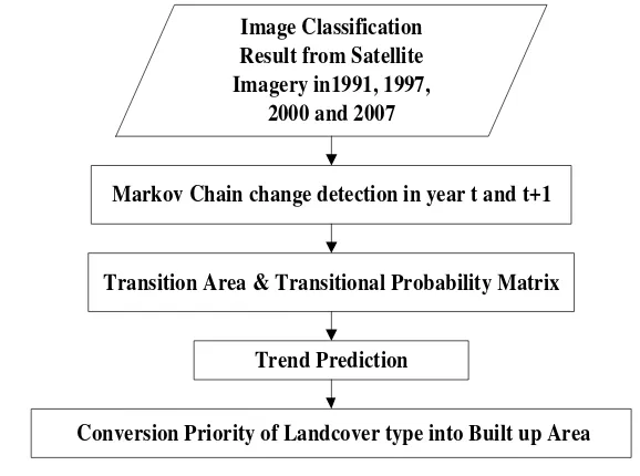
In this research, markov chain change detection used to get landcover type
priorities conversion to urban build up area based on matrix probabilities. The
calculation process can be explained in Figure 2.2.
Markov Chain change detection in year t and t+1
Transition Area & Transitional Probability Matrix
Trend Prediction
Conversion Priority of Landcover type into Built up Area Image Classification
Result from Satellite Imagery in1991, 1997,
[image:36.595.162.451.211.426.2]2000 and 2007
Figure 2.2 Priority of Conversion using Markov Change Detection
In the first step image classification processed using visual interpretation
methods was done. The result from this processed can be divided into seven class
type of landcover, there are ; built-up area, forest, paddy field, plantation,
agricultural, shrub and water body.
Second step is to create a transition matrix of pixels in each class for two
times. This is the same as the cross tabulation matrix, which can be used for
accuracy assessment. From this step, trend prediction will be calculated using
matrix probabilities. Landcover priorities scenarios can be derived from
transitional probabilities of landcover type in year t that changed into built-up area in year t+1. Afterwards, the value of probabilities has been ranked from higher to lower probabilities. This step was done to get decision of landcover type
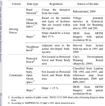
19 2.3.3.Calculation of Driving Forces
Data collection and regulation of driving forces and constraints for urban
development was get from official agency. The regulation and source of the data was
[image:37.595.81.513.197.634.2]given in Table 2.5.
Table 2.5 Driving forces and constraints regulation for urban development
Criteria Data type Regulation Source of the data
Driving Forces
Road Network1)
Closer the distances
from the roads Bakosurtanal, 2000
Urban Hierarchy Index 1)
Based on the number and types of facilities that are located within the region
Village potential statistics & Statistical year book for Bandung area in 1991 and 200.
Slope 1)
Slope should be a lower than 15 %
DEM from SRTM Imagery with spatial resolution 90 m.
Neighbour hood1)
Adjacent area to the actual developed built-up area
Derived from Actual built-up area in 1991 and 2000
Constraints
Protected Forest2)
Not located in Protected forest and Water Body area
City's Development Planning Board (Bappeda, 2000)
Water body, Open Green space 1)
Not located in Protected forest and Water Body area
Classified from Landsat TM 1991 and 1997, and references map from Bakosurtanal, 2000 and BPN,2007.
Slope 1) Slope > 15 %
DEM from SRTM Imagery with spatial resolution 90 m.
1) According to ministry of public works SNI 03-1733-2004 about codes of housing design in urban areas.
2) According to KEPPRES No.32 year’s 1991 about protected area.
1) Neighbourhood Effect
Urban development usually takes place first in the adjacent area to the
developed urban area. That is where CA model can make sense. Considering only the
20 N fx y, ( ,q Num) (1.5)
Where f (q,Num) is a function of the neighbourhood for cell in location (x,y), q
is the developed cells in the neighbourhood and N is the number of the neighbours. The simplest way to define this is to use the q as the amount of developed cells in the neighbourhood and use Num as the total number of its adjacent cell in its neighbourhood. In this sense, f is define as
, /
x y
f q Num (1.6) Where q is the number of developed cells in the neighbourhood in this case
existing urban cell and Num is the total cell number of the neighbourhood. In this
research, 3 x 3 moore neighbourhood was applied, so equation 2.6 can be expressed
as :
3 3 ,3 3 1 ij x y
con S urban f
(1.7)Simple IF…THEN rules are used to drive the simulation IF the tested cell is urban, THEN keep it urban
IF the tested cell is non-urban THEN equation 2.7 will be applied IF the tested cell is constraint, THEN keep it no change.
2) Urban Hierarchy Index (UHI)
Scalogram method was used to calculate UHI. The equation used is :
n k k k k k n HI F a
(1.8)Where :
k
HI : Hierarchy index in sub district - k
k
F : Number of Availabele types in district - k
k
a : Number of Availabele types in district - k
k
21 Village potential statistics data in 1991 and 2000 was used to calculate the UHI,
the process was shown in Table 2.6.
Table 2.6 UHI Processing
No District Sub
district
Popula tion
Facilities Total
Facilities Hierarchy
Indeks
F1 F2 F3 ...Fk...
n k k
F
1 A A1 ... .... .... .... ...
2 A A2 ... .... .... .... ...
3 B B1 ... .... .... .... ...
- ... ... ... .... . .... . .... . ...
i i i ... .... .... .... ...
Number of types a1 a2 a3 ...ak...
Number of facilities n1 n2 n3 ...nk...
Weighted 1
1 n a 2 2 n a 3 3 n a k k n a
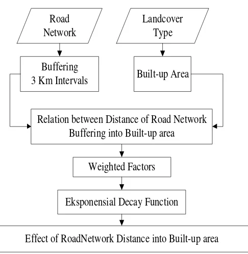
3) Road network effect
The road network effect is usually calculated in terms of accessibility. In the
case of the exponential decay function, the equation used is:
1 ij n d i j j
T
W e
(1.9)Where Ti is the accessibility of cell i, W is the weight for road class j, dtjis the distance from cell i to the nearest road class j, β is the exponent. The common concept on accessibility is that the effect of road, which influences the location choosing
process for residential area, is a function of power exponential decay. Weighted
calculation in equation 2.9 was calculated by overlaying between urban area and the
result from reclassification process at a specific distance from road network. In this
case, buffering proses was assumed at 3 km from road network. Figure 2.3 show this
22 Road
Network
Buffering 3 Km Intervals
Landcover Type
Built-up Area
Relation between Distance of Road Network Buffering into Built-up area
Weighted Factors
Eksponensial Decay Function
[image:40.595.194.437.78.327.2]Effect of RoadNetwork Distance into Built-up area
Figure 2.3 Calculating of Road Network Effect
4) Slope Effect
In this study, regulation are being used for slope criteria base on ministry of
public works SNI 03-1733-2004 about codec of housing design in urban areas,
should be less than 15 % for urban developmnet.
Figure 2.4 The expected relation between slope and urban land
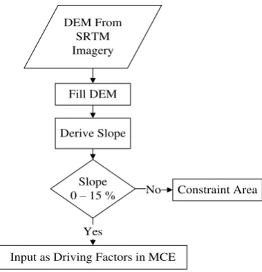
Slope derivation from DEM and how to get constraint area from slope
processing, explained in a diagram in Figure 2.5.
0 Slope (%) 15
Ur
b
an
De
v
elo
p
m
en
tt Maximum Slope
[image:40.595.232.430.490.631.2]23
DEM From SRTM Imagery
Fill DEM
Derive Slope
Slope 0 – 15 %
Input as Driving Factors in MCE
Constraint Area
Yes
[image:41.595.217.407.82.279.2]No
Figure 2.5 Slope derivation from DEM
2.3.4.Multi-criteria Evaluation of Driving Forces.
Multi-criteria evaluation (MCE) was used to evaluate the driving forces by
combining or overlaying each criterion. In this research, slope, road network effect,
hierarchy index and neighbourhood effect as criteria of driving forces. The first step is
standardized each criterion score into range 0 – 1. Figure 2.6 show this processes.
Driving Factors
- Neighbourhood Effect - Slope Effect
- Distance From Road Network - Urban Hierarchy Index
Liner Trasformation Scale into 0 -1
Standarized Value for each Driving Factors Development of
Built-up Area 1991 - 200
Mean Value for each driving factors related to Built-up area development 1991 - 2000
Weighted calculation using Ranking Methods
Weighted Factors For each driving Factors
Allocation of Potensial Cell Suitability for Built-up Area Area using MCE
Overlay
Built-up Area 1991
Built-up Area 2000
Erase
[image:41.595.88.499.451.703.2]24 The linier scale transformation methods was used to get standardized score
from each criteria. The most often used procedure in this methods here are maximum
and minimum score and the score range procedure (Voogd 1983; Massam 1988).
Equation 2.10, was applied to get standardized criterion score.
max max min j ij ij j j
x
x
x
x
x
(1.10)Where :
'
ij
x : Standardized score for theobject-i andattribute - j
ij
x : Raw score
max
j
x : Maximum score for the jth attribute min
j
x : Minimum score for the jth attribute
The seconds step is overlaying or combining each criterion, after the linier scale
transformation was applied. The last process in this step is weighted calculation.
Ranking methods will be used to create the importance weighted from each criterion.
In the ranking methods, rank sum is one of popular approach (Stillwell et al, 1981). This method will be used to calculate the weighting for each criterion and can be
formulated as:
1
1
j i kn r
w
n r
(1.11)25 2.4. Result and Discussion
2.4.1.Data Preparation and Processing of Driving Forces
Neighbourhood effect, distance to road, UHI and slope with the value less than
15% were used as a driving forces for urban growth development. Neighbourhood
effect was simulated from actual urban in 1991 to get neighbourhood value in year
2000. Village potential statistics data in 1991 and 2000 was calculated using
scalogram methods to get value of UHI. Distance from road was calculated using
exponential decay function, whereas slope less than 15% was derived from DEM
SRTM with spatial resolution 90 M. Constraint area in the study area including:
protected forest, slope greater than 15% , open green space and water body. All of the
data has been converted into raster data with spatial resolution 100 x 100 m, and then
converted again to point vector data. The linier scale transformation method was
applied to get standardized score from each criteria. The result from this calculation
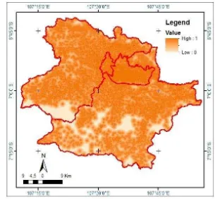
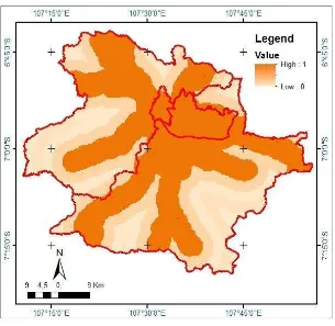
are all of the data value will be range from 0 – 1 which 1 is maximum value. Figure 2.7 until 2.10 was shown spatial distribution of driving forces. Whereas, Figure 2.11
[image:43.595.155.460.438.720.2]was shown constraints area in study area.
26 Figure 2.8 Road Network Effect
27 Figure 2.10 UHI Effect
28 2.4.2.Weighting Factors Calculation of Driving Forces
Map overlay technique using intersection between developments of built-up
area in 1991- 2000 and driving forces (neighbourhood effect, UHI, Slope and
Distance from Road) were used to get average value for each driving forces. Ranking
method was applied to calculate of weighted for each driving forces. Table 2.7 show
the result and calculation process to get weighted for each driving forces.
Based on the result of weighted calculation in Table 2.7, neighbourhood effect
is the most important influence factors in built-up area development during 1991 – 2000 in study area. The weighted was contributing 48% for urban development. This
condition was agreed with the theory, urban development usually takes place first in
the adjacent area to the developed built-up area. The others important influences
factors in built-up area development process are distance from road, UHI and slope.
Closer the distances from the roads having an effect to increase new development of
up area. This condition was contributing about 24% weighted influence in
built-up area development during 1991 - 2000.
Table 2.7 Weighted for Driving Forces using Ranking methods
Driving forces Average
Rank Sum
Straight Rank
Reciprocal Weight
(1/rj)
Normalized Weight
Neighbourhood Effect 0.786 1 1.000 0.48
Urban Hierarchy Index 0.591 4 0.250 0.12
Slope 0.638 3 0.333 0.16 Road Network Effect 0.705 2 0.500 0.24
Total 2.083 1
Ordinarily, built-up area will grow where there are flatten areas. In this study,
slope effect was contributing 16 % weighted influence in built-up area development.
Amount of services facilities and number of public facilities in a region is once factor
that affected in build-up area development. Scalogram method was applied to derive
urban hierarchy index based on amount of services and number of public facilities in
a region. The result from urban hierarchy index analys