THE CHOLESKY UPDATE FOR UNCONSTRAINED OPTIMIZATION

THE CHOLESKY UPDATE FOR UNCONSTRAINED OPTIMIZATION

Saad Shakir Mahmood

College Of Education, Department Of Mathematics Almustansiriya University

Email: saadshakirmahmood@yahoo.com

ABSTRACT

It is well known that the unconstrained Optimization often arises in economies, finance,

trade, law, meteorology, medicine, biology, chemistry, engineering, physics, education, history,

sociology, psychology, and so on. The classical Unconstrained Optimization is based on the

Updating of Hessian matrix and computed of its inverse which make the solution is very

expensive. In this work we will updating the LU factors of the Hessian matrix so we don’t need to

compute the inverse of Hessian matrix, so called the Cholesky Update for unconstrained

optimization. We introduce the convergent of the update and report our findings on several

standard problems, and make a comparison on its performance with the well-accepted BFGS

update.

Keywords : Unconstrained Optimization, Cholesky Factorization, Convergence

ABSTRAK

menggunakan penyesuan tersebut, kemudian kami memandingkan hasil yang kami dapat dengan hasil dari penyesuaian BFGS yang terkenal pada masalah potimasi tak berkendala.

Kata Kunci : Unconstrained Optimization, Cholesky Factorization, Convergence

INTRODUCTION

Given f :Rn →R, it is assumed that: 1. f is twice continuously differentiable. 2. f is uniformly convex, i.e., there are m1

and m₂ >0 such that

2 2 2

2

1 a a fa m a

m ≤ T∇ ≤ , were

" R a∈ .

The method proposed by Hart (1990) is to update the Jacobian matrix of f on the basis of both L' unit lower triangular and U' upper triangular matrices. He takes

' 'U L

B= the current approximation of Jacobian matrix and he defines

) ' )( '

(L O U Q

B+ = + + , with the updating matrices O and Q lower triangular and upper triangular, respectively. Then he determines O and Q from the following relations:

r s Q U

y r O L

= +

= +

) ' (

) ' (

and he used the following elementary lemma to solve the above system:

LEMMA

If β∈R and a∈R" such that aTa≠0, then the minimum value of xTx= x₂, such that

β

= x

aT is

a a

a x=β _T .

The update satisfies the Quasi-Newton condition but it’s not symmetric.

THE CHOLESKY UPDATE

Given f :R"→R, suppose that B is the current approximation of the Hessian matrix, and B+ is the next approximation of the Hessian matrix. Suppose also that B is positive definite. There exists matrices L' and U'∈Rn×n, with 'L unit lower triangular matrix and U' upper triangular matrix, such that

' 'U L

B= (1)

then L+ and U+ are to be updated, such that

L+ =L'+O (2) Q

U

U+ = '+ (3)

+ + +₌

U L

B (4)

Since B is symmetric then there is a diagonal matrix D such that

T DL

U'= ' (5) and B=L'DL'T

T L D D L

B= ' 21 21 '

with                   = nn d d d D . . 0 0 0 . . . . . . . . . . . . 0 0 . . 0 22 11 2 1 Hence T L L

B= (6)

with 2

1 'D L

L= , and O=QT so (4) becomes

T

L L

B+= + + (7) by the Quasi-Newton condition it follows

y r L+ =

r s

L+T = ₍₈₎

with n

R

r∈ _{, from (8)}

y s s B s s L L s r

rT = T + +T = T + = T

(9) so the best choice of r which guarantees convergence is s L s B s y s

r _T T

T

= . (10)

The solution of system (8) is obtained by using the elementary lemma as follows: i j n i r r y l _n i k k j i

ij , 1, 1 and 1,

2 = − = =

∑

=

+ ₍₁₁₎

n j s s l r l n n j k k kj j

nj , 1, ,

1 * = − =

∑

− = + (12) It is clear that the update is symmetric. In order to show that the update satisfies the Quasi-Newton condition, the following lemma is introduced:

Lemma 1

The Cholesky update given in (11) and (12) satisfies the Quasi-Newton condition.

Proof:

It is only needed to show that

∑

n n

n n n

T n n

y s

s y s

s y s y s

y s y

= =

+ −

− − −

= 1 1 2 2 −1 −1

THE CONVERGENCE OF THE

UPDATE Assumption I

(a) ∇f :R"→R" is continuously differentiable in an open convex set D, (b) there is an x* such that ∇f(x*)=0 and

) ( *

2

x f

∇ is nonsingular,

(c) there is a constant K and p>0 such that ∇2f(x)−∇2f(x*) ≤K x−x* p, In proving a convergence result of the same nature as for other Newton-like methods, a Lipschitz condition is assumed on the Hessian matrix. Using factorization and an open pivoting strategy, the factorizations must be shown to be continuous. This has been established in Dennis and Schnabel (1983).

Definition 1:

Let M_L =

{

M∈L

( )

Rn :m_ij =0,1< j

}

lower triangular matrices. Furthermore let the following mapping be defined:

( )

L

n

L LR M

L : →

such that LL

( )

M =M .

Lemma 2 (Royden 1968)

i. Mx ₂≤ M _F x₂;

ii. M _F ≤cM ₂ for some c>0; iii. M _F = LL

( )

M _F

Definition 2

Let L L

n

M M

R × →

:

φ , and Let

) ,

(x* L* be an element of R"×ML. The update function φ has the bounded deterioration property at

( )

* *

,L

x if for some neighborhood D1×D2 of

( )

* *

,L

x there exist constants α₁ and α₂ such that if

) ( ,

1 LL s f x D

x∈ T =−∇ and x+ =x+s, then for any L+∈φ

( )

x,L .

[

1 ( , )

]

* ( , )

* ₁ + ₂ +

+ _{−L ≤ + x x L−L + x x}

L ασ α σ

where

   



 _{− −}

= +

+ _p p

x x x x x

x, ) max * , *

(

σ

.

Assumption II

Let ∇2f(x*) be LLT - factorable, i.e.

T

L L x

f( *) * *

2 =

∇ , where L*∈ML, is

invertible, and ∇f(x*)=0.

Let L∈M_L, and δ,γ >0 satisfy (i) L−L* ≤2δ <1,

(ii) max

{

L*, L*−1, ∇f(x*)

}

≤γ. Then each of the following holds: (a) L is invertible and

γδ γ

2 1 1

− ≤

−

L ,

(b) L ≤2δ +γ ,

(c)

δγ γ δγ

2 1

1 2 * *

2 1

1

− + ≤

− −

− T T

L L L

L ,

(d) LLT −L*L*T ≤4δ(2δ +γ).

Note that, this technical lemma involves some useful norm inequalities. Since the lemma (and the proof) is independent of the way the lower triangular L is used, it is the choice to use L within the context of the Cholesky update. The inequality (c) is thus of no special interest. However, (d) is needed to represent the addition to the original lemma. The proof for (d) is straightforward.

Theorem 1

Let f satisfy assumption I, and assume that the update function φ satisfies the bounded deterioration at

(

x*,L*

)

. If for any p∈

[ ]

0,1, there exists an ε =ε

( )

r and δ =δ

( )

r such that

(i) x0−x* <ε, (ii) L₀−L* ≤δ,

(iii) L+∈φ

( )

x.L ,

then the sequence

{ }

xk , defined by )

(

,

1 x s LL s f x

xk+ = k + k T =−∇ satisfies for each k≥0,

xk+1−x* ≤ p⋅ xk−x* ; Moreover, each of _{L, L}−1

is uniformly bounded.

Proof

Let p∈(0,1). Choose a neighborhood D1×D2 guaranteed by the bounded deterioration property, and restricted so that it contains only invertible matrices. Given c in lemma 2, and γ as in lemma 3, choose ε(p) and δ(p) such that

2 1 ) ,

(x L ∈D ×D whenever x₀−x* <ε and

δ

2 * ≤

−L

L , such that

(

)

[

(

)

]

(

)

(13) 1

2

4 2

1 1 2

2 1

2 2

δ ε

α δ α

γ δ δ ε γδ δγ

≤ − +

≤ + +

− <

p p p

r

p K

r

where α1 and α2 are determined by D2 and the bounded deterioration property. First, it is to be noted that

( )

( )

( )

( )

*)] *))(

( (

*) (

*

* [

* *

0 2

0 0

0 2

0 1 0 0

0 1 0 0 0

1 1

1

x x x f L

L

x x x f

x f x f L L

x f L L x x x x

T T

T

− ∇

−

− − ∇

− ∇

− ∇

− =

∇ −

− = −

−

−

−

−

[

]

[

]

*

* )

2 ( 4 )

2 1 (

* )

2 ( 4 *) , ( *

0

0 2

2

0 0

1 0 0 1

1

x x

x x K

r

x x x

x K L L x x

p T

− ≤

− +

+ −

≤

− +

+ ≤

− −

ρ

γ δ δ ε γδ

α δ δ σ

Thus x1−x* ≤ε and x1∈D1. By way of

induction. Assume that for

1 , , 2 , 1 ,

0 −

= m

k , then L−L* ≤2δ, and *

*

1 x x x

xk+ − ≤ρ k− .

Then by the bounded deterioration property and the fact that

(

x_{k 1},x_k

)

max x_{k 1} x*p, xk x* p ρpkεp,

α ≤

   



 _{− −}

= +

+

it following

. 2

*

* 1 2

1

p pk p

pk

k L L L

L ₊ − − − ≤ αδρ ε +α ρ ε summing both sides from k=0 to m−1, a telescoping sum on the left is obtained and thus

δ ρ ε α δ

α ) 2

2 ( * *

1

0 2 1

0− + + ≤

≤

−

∑

−

=

m k

pk p

m L L L

L

Hence, by the technical lemma, and

γ δ + ≤2 m

L . It follows analogously to the case m=1 that

* *

1 x x x

xm+ − ≤ρ m−

Observe that for any ε >0, there is a δ >0 such that if x−x* <ε and L−L* ≤2δ

then the computed iterate

) ( )

(LL 1 f x

x

x+ = − T − ∇ must satisfy

*

* x x

x

x+− ≤ − . Lemma 4 (Bartle 1975):

Let

{ }

xn be a sequence of positive real numbers. Then

∑

n n

x converges if and only if the sequence S=

{ }

sn of partial sums is bounded.

Lemma 5 (Bartle 1975):

If

∑

n

n

x converges, then lim =0 ∞

→ k

k x .

Now in this direction the following result will be needed. The straightforward proof is omitted.

Corollary 1 (Dennis and Schnabel, 1983) If f satisfies the assumptions I and II then for any ε >0, there is a neighborhood D_ε of (x*,L*) such that if

ε

D L x, )∈

( , then σ(x,x+)<ε . Corollary 2

Define η = y−Lr, with r computed from the Cholesky update which satisfies

y r

L+ = . Then η =Ty with T lower triangular, bounded, and T*=(L*)−1.

That η =Ty and T lower triangular are obvious. The bounded- ness comes from the fact that it is invertible and L satisfies the hypothesis of theorem 1. The fact that T*=(L*)−1 is obtained by direct substitution.

In order to obtain bounded deterioration property for the update,

bound on

[

]

T

n r r

r r v n i

v₁, =1,2,3, , , ₁= _{1 2 3} . . . is required. In particular, v₁ must approach to zero at essentially the same rate as s .

Lemma 6 (Byrd and Nocedal, 1989). Under assumption I, it follows

. and for ,

,

2 2

2

R M m

M s y

y M s s y s

m ≤ T ≤ _T ≤ ∈

Lemma 7

Let f satisfies the assumption I. Let vi defined as vi =

[

r1 r2 . . . ri

]

T There exist numbers ε,ρ1 and ρ2 such that if

ε

σ + <

) ,

(x x , then

. , , 3 , 2 , 1 , 2

1 i n

v s

i

= ≤

≤ ρ

ρ

Proof

By the Cholesky update s y r r

r r

rT = + 2+ + _n2 = T 2

2

1 (14)

and from (14)

s y r r

v T

n k

k i

k k

i =

∑

≤

∑

=

= =

2

1 2

,

thus by

Lemma 6,

p

M s M v_i

1

ε

≤ ≤

thus

i v M p

1 1

1 ≤

ε , and so

i n

v s

M s

M s

p p ≤ ≤

2 1

2

ε

ε .

If we set

p

M sn

1 2

1

ε

ρ = then

i v

s

≤

1

ρ (15)

Since

∑

=

≤ i

k k r r

1 2 2

1 , then

∑

=

= n

k k kl T

T

s l s B s

s y r

1 2

1 , by Theorem 1 L is

boded, and hypothesis p

s

1

ε

≤ , so there is a number ξ_ij >0 such that l_ij ≤ξ_ij for all i and

j, and such that i

n i

n k

ki T

T

v s

B s

s y

p ≤

∑∑

=1 =1 1

ε ξ

By lemma 6, and the boundedness property of L and s , exist a number ζ >0 such

that _i

n i

n k

ki v

s

m _p

≤

∑∑

=1 =1 1

ε ξ ξ

Since sn ≤ s , then it follows

i n

i n k

ki n

v

ms _p

≤

∑∑

=1 =1 2

1

so,

∑∑

= = ≤ _n i n k ki n i p p ms v s 1 1 2 1 1 ε ξ ζε

The Lemma thus holds by letting

∑∑

= = = _n i n k ki n p p ms 1 1 2 2 1 1 ε ξ ζε ρ Lemma 8

Let f satisfies the assumption I. Let i

v defined as vi =

[

r1 r2 . . . ri

]

T. There exist numbers '

1

,ρ

ε and ' 2

ρ such that

if σ

( )

x,x+ <ε , then ρ1≤ ≤ρ2 i v

r

. Proof

By lemma 6, and lemma 7

' 2 2 1 ' 1 ρ ρ ρ ρ = ≤ ≤ ≤ ≤ = M v s M v s y v s m m i i T i

Now, in order to proceed with the main objective, the following abbreviation is introduced.

(a) v_i =

[

r₁ r₂ r₃ . . . r_i

]

(b) C=L−L*,C+ =L+−L*, (c) α =Ty−LTs,α*=T*y−LT*s, (d) β=Cr,

consequently, (e)                 −         − = + 2 2 * i T L i T L v r L v r L C

C β α

Lemma 9

Let f satisfies assumption I and II. Let α* be as above. Then there exist numbers

0

>

K and ε >0 such that if σ

( )

x,x+ <ε

then

(a) K

( )

x x i n

v_i i , , 2 , 1 for , , ' * = ≤ _σ + α

(b) _ ≤

( )

+

      x x K v r L F i T

L " ,

*

2 σ

α

.

Proof

Since α*=T*y−LT*s=T*

(

y−∇2f(x*)s

)

, if T_i* is the i-th row of T*, then

(

y f x s

)

T_i

i* * ( *)

2

∇ − =

α , giving

s x x K T s x f y T i i i ) , ( * *) ( * * 2 + ≤ ∇ − ≤ σ α

By lemma 7 there exist ρ>0 and ε >0 such that if σ

( )

x,x+ <ε and

( )

+ _{≤ ⋅}

( )

+

≤ K T x x

v s x x T K

v i F

i F i i i , * , * * σ ρ σ α

this proves (a) with K'=KρT*_F. Now, to prove (b), let

        = ₂ * * i T i L v r L A α

( )

( )

( )

(

)

( )

+ + = = = ≤ ≤         = = =         =

∑

∑

∑

x x K n A x x K v r A v A v v A v r A F n i n i _i j i F i i i i i i i i i j _i j i i , ' * , ' * * * * * * * * 2 1 2 2 1 2 2 2 2 2 2 4 2 2 2 1 2 2 σ σ α α α α

this proves (b) with K"= nK'.

Lemma 10

Let f satisfies the assumption I and II. Then the Cholesky update algorithm satisfies

( )

C+ ≤

(

1−

)

C +K'

( )

x,x+ , F

F θ σ

where 1

( )

0,1.

2 ∈         = i v C β θ Proof

Let _

      − = ∇ + 2 * i T L v r L

C α . Then

, of row th the denotes if Thus, . 2 ∇ ∇         − = ∇ i v r L C i i T L β

∑

∑

∑

∑

∑

∑

∑

− = ∇ + − = ∇ + − = ∇                 + − = ∇         − = ∇ = = = = 2 2 2 2 2 4 2 2 2 2 2 1 1 2 4 2 2 2 2 1 2 2 2 2 2 2 1 2 2 2 2 2 i i ij i i i i i i ij i i j i j j i i j ij i i ij i i j _i j i i j i ij ij i i j _i j i ij i v c v v v c r v r c v c v r v r c c v r c β β β β β β β β thus,

∑

∑

∑

∑

∑

= = = = = − = ∇ < − = ∇ = ∇ n i _i i F F n i n i _i i i j ij n i i F v C v c 1 2 2 2 2 1 1 2 2 1 2 1 2 2 0 β β observe that 2 1 2 2 0 _F n i _i i C v < <

∑

= β thus, setting

∑

= = n i _i i F v C 1 2 2 2 1 β θ

gives 0≤θ ≤1.

,and so by lemma 9,

Let f satisfies assumption I and II. Then there exists a neighbourhood D₁×D₂ of

(

x*,L*

)

such that in D1×D2 the update function φ

( )

x,L described above is well defined and the corresponding iteration

( )

, 1 1

x f L L x

x+ = − T− −∇

where L+ =φ

( )

x,L is locally convergent at *

x .

Proof

Set =

( )

− ₊ x x, 1 1

σ θ

α , and α2 =K'. Then by

lemma 7

( )

( )

( )

[

+

]

( )

+

+

+ +

+

+ +

≤

+ ≤

x x C

x x C

x x C

x x C

, ,

1

, ,

2 1

2 1

σ α σ

α

σ α σ

α

So the Cholesky update function φ

( )

x,L satisfies the deterioration property and the convergence follows from theorem 1.

Corollary 3

Assume that the hypotheses of Theorem 2 hold. If some subsequence of

{

Lk −L*_F

}

converges to zero, then

{ }

x_k converges q-superlinearly to *x .

Proof

It is necessary to show that 0

* =

−

∞

→ k F

k L L

Lim

From the proof of Theorem 1 ,

2

* ≤ δ

− _F

k L

L

δ is defined in Theorem 1, therefore

F

k L

L − * is bounded above and by Lemma 4, converges, and by Lemma 5,

0

* =

−

∞

→ k F

k L L

Lim . Now it is necessary to

show that 0.

* *

lim 1 =

− −

+ ∞

→ _{x x}

x x

k k k

Let h∈

( )

0,1 be given. By Theorem 1 there are numbers ε

( )

h and δ

( )

h such that

( )

h L

L₀− *_F <δ and x₀−x* <ε

( )

h which imply that x_k+1−x* ≤h x_k−x* for each

0

≥

k . However, if m>0 is chosen such that

( )

h L

L_m− *_F <δ and x_m −x* <ε

( )

h and thus, x_k+1−x* ≤hx_k −x* for each k≥m.

So ,

* * 1

h x x

x x

k

k _≤

− −

+

and since h∈

( )

0,1 was

arbitrary, then 0.

* *

lim 1 =

− −

+ ∞

→ _{x x}

x x

k k k

NUMERICAL RESULTS

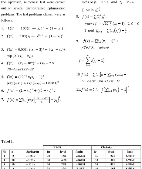
this approach, numerical test were carried out on several unconstrained optimization problems. The test problems chosen were as follows:

1. = 100 — + 1 − . 2. = 100 — + 1 −

.

3. = 0.0001 ( − 3 − ( − )+ exp (20 ( − )).

4. = − 10 + − 2 × 10−62+ 1 2−22.

5. = 10 − 1 +

[ − + − − 1.0001] .

6. = 1 − + − .

7. = ∑ ! "# $%

"& ' − ()*

++

), ,

.ℎ 0 () = 0.1 1 234 5) = 25 +

[−50 ln ()]

% # . 8. = ∑9:_{), )} ,

;ℎ 0 ) = √10 = )− 1 , 1 ≤ 1 ≤

3 234 9: = ∑ ?9@, @A − .

9. = ∑9_{), )} − 1 + 2+ 3 , ;ℎ 0

= B C? @− 1A. 9

@,

10. = ∑ D3 − ∑ EFG9), 9@, @+ 11−EFG 1−G13 1+ 1−12. 11. = ∑ 1 H∑ C9 @

@, I − 1' . 9

[image:11.595.51.519.118.675.2]

),

Tabel 1.

BFGS Cholesky

No n Starting point Itr feval f min Itr feval f min

1 2 (-1.2,1) 30 188 4.86E-8 35 221 6.65E-9

1 10 (-1.2,1) 30 -428 4.86E-8 35 501 6.65E-9

1 20 (-12,1) 30 728 4.86E-8 35 851 6.65E-9

2 2 (-1.2,1) 31 195 7.11E-8 26 159 5.29E-6

2 2 (-3.635,5.621) 132 803 3.205E-10 35 229 2.03B-5

2 2 (639,-0.221 280 1818 339E4 44 263 6.13E-10

3 2 (0,0) 5 29 0.2008 5 29 0.2008

3 2 (30,30) 13 81 0.1998 3 17 0.2723

4 2 (1,1) 27 241 1.35E-6 24 201 4.87E40

4 2 (10,-0.5) 248 1280 3.69E-7 27 214 5.49E-11

4 2 (100,100) 392 1928. 3.14E-8 32 260 1.96E-10

5 2 (0,1) 3 16 0.9999 3 16 0.9999

5 2 (0.01,5) 2 9 1 2 9 1

5 2 (3,-0.5) 3 16 -1 3 16 1

6 3 (2,4,2.5) 10 63 2.09E-4 10 68 2.23E-4

6 3 (0.6,6,3.5) 8 53 235E-6 14 91 3.06E-6

6 3 (0.7,5.5,3) 9 59 2.68E-5 12 87 1.03E-5

7 3 (250,03,0) 14 99 7.13E-4 13 91 7.92E-4

7 3 (25,-2,0) 1 4 2.8393 1 4 2.8393

7 3 (200,0.1,40) 17 123 3.20E-4 15 110 3.20E-4

8 10 (1,2,3,…) 5 70 7.60E-5 5 70 7.62E-5

8 20 (1,2,3,..) 17 414 9.47E-4 7 168 2.46E-4

8 30 (1,2,3,..) 53 1817 3.04E-4 265 9047 2.27E-4

8 10 -(1,2,3,..) 5 70 1.34E-4 5 70 '133E-4

8 20 -(1,2,3,..) 17 412 1.67E-4 8 - 199 1.68E-4

8 30 -(1,2,3,…) 59 2022 3.13E-4 188 6031 3.53E-4

9 20 1 – iln 25 604 2.20E-9 8 195 6.62E-9

9 30 1 – iln 91 3340 4.82E-10 9 309 132E-9

9 40 1-i/n Filed Filed Filed 14 145 6.51E-9

9 20 1 - i/2n 11 274 3.50E-11 8 191 6.18E-9

9 30 1 - il2n 100 3360 1.63E-9 12 400 6.01E-10

9 40 1 - il2n 101 4550 2.08E-11 9 402 2.27E-10

10 10 (1,2,3,..) 90 1280 29.0596 1357 17143 9.2360

10 20 (1,2,3,..) 19 269 36.2260 1549 21175 4.7698

11 10 (1,2,3,..) 3 55 2.1429 2 25 2.1429

11 20 (1,2,3,..) 97 2089 4.6341 6 79 4.6341

11 30 (1,2,3,..) 113 3327 7.1311 3 107 7.1311

11 10 -(1,2,3,..) 2 25 2.1429 2 25 2.1429

11 20 -(1,2,3,..) 90 2019 4.6341 4 90 4.6341

11 30 -(1,2,3,..) 96 3003 7.1311 3 106 7.1311

CONCLUSION

Hart update is satisfying the Q-N condition but it's not symmetric, and since the Hessian matrix is symmetric so to preserve the symmetric property is very important. From equation 11 and equation 12, clear that the cholesky update is satisfying Q-N condition and preserve the

see that the Cholesky update with large dimension has a good results

REFERENCES

Byrd R. H. and Nocedal J. 1989. A tool for the analysis of quasi-Newton methods with application to unconstrained minimization. SIAM J. Number. Anal., 26: 727-739

Bartle R. G. 1975. The elements of real analysis. Wiley international edition. USA. 286-330 David G. Luenberger and Yinyu Ye. 2009. linear and Nonlinear Programming. Third Edition.

Springer

Dennis J. E. and Schnabel R. B. 1983. Numerical Methods for Unconstrained Optimization and Nonlinear Equations. Prentice-Hall, Inc., Englewood Cliffs, New Jersey.

Hart, W. E. 1990. Quasi-Newton methods for sparse Nonlinear system. Memorandum CSM-151, Department of Computer Science, University of Essex.

Royden, H. L. 1968. Real Analysis. second edition, Macmillan Publishing co. INC. New York. Saad S.. 2003. Unconstrained Optimization Methods Based On Direct Updating of Hessian

Factors. Ph. D. Dissertation. Gadjah Mada University. Yogyakarta, Indonesia.