FORECASTING LAND USE CHANGE AND THE IMPACT
ON WATER YIELD AT WATERSHED SCALE
YUSUF RAHADIAN
GRADUATE SCHOOL
BOGOR AGRICULTURAL UNIVERSITY B O G O R
STATEMENT OF THESIS AND INFORMATION SOURCES
Hereby I declare the thesis entitled Forecasting Land Use Change and the Impact on Water Yield at Watershed Scale, is result of my own work under supervision of supervisory committee and it has not been submitted yet in any form in any university to obtain a degree. The researcher has full responsibility for all contents of this thesis. Sources of information derived or quoted from other researchers, whether it is published or not are mentioned in the text and listed in the bibliography at the end of this thesis.
Bogor, January 2014
ABSTRACT
YUSUF RAHADIAN. Forecasting Land Use Change and the Impact on Water Yield at Watershed Scale. Supervised by SURIA DARMA TARIGAN as supervisor and IBNU SOFIAN as co-supervisor.
The focus in this study is on the impact of land-use changes from 1991 until 2030 on the water yield quantity in Upper Cisadane Watershed. This study tests a methodology, which involves coupling a land-use change model with a hydrology model. The future land-use is modelled with the CLUE-S model. Four scenarios are developed based on land use demand (population growth) and area restriction (spatial policy). Hydrology components, in case of water yield is simulated using the HEC-HMS model. Result from land use model show that trends of land use changes of the area during 1991 – 2030 depict grassland, settlement and forest area are increasing over time, whereas estate tend to decrease and water remains constant. Based on hydrology model simulation shows increasing of water yield from Year 2010 to Year 2030. The increasing values of water yield influenced by forest rehabilitation activity by the government inside forest area and the development of community forest outside the forest area. Increasing values of water yield are higher for scenario 2 and scenario 4, where government policy about restriction of land use inside forest area applied. That means government policy to prohibit land use conversion inside forest area is appropriate to apply.
ABSTRAK
YUSUF RAHADIAN. Forecasting Land Use Change and the Impact on Water Yield at Watershed Scale. Di bawah bimbingan SURIA DARMA TARIGAN sebagai pembimbing I dan IBNU SOFIAN sebagai pembimbing II.
Fokus dari penelitian ini adalah mengenai dampak perubahan penggunaan lahan pada periode tahun 1991 – 2030 terhadap produksi air di Daerah Aliran Sungai Hulu Cisadane. Penelitian ini menguji sebuah metodologi yang merupakan kombinasi antara model perubahan penggunaan lahan dengan model hidrologi. Penggunaan lahan di masa depan dimodelkan dengan CLUE-S. Empat skenario dikembangkan berdasarkan permintaan penggunaan lahan (pertumbuhan populasi) dan pembatasan wilayah (kebijakan spasial). Komponen-komponen hidrologi, dalam hal ini produksi air, disimulasikan dengan menggunakan model HEC-HMS. Hasil dari pemodelan penggunaan lahan dalam jangka waktu 1991-2030 menunjukkan tren perubahan penggunaan lahan padang rumput, area terbangun, dan hutan bertambah, sementara area perkebunan menurun, dan badan air tetap. Hasil simulasi model hidrologi menunjukkan peningkatan produksi air pada periode 2010-2030. Peningkatan produksi air dipengaruhi oleh aktifitas rehabilitasi hutan oleh pemerintah di dalam kawasan hutan dan pembangunan hutan rakyat di luar kawasan hutan. Peningkatan produksi air lebih tinggi pada skenario 2 dan skenario 4, di mana kebijakan pemerintah mengenai larangan konversi penggunaan lahan di dalam kawasan hutan diimplementasikan. Artinya, penerapan kebijakan pemerintah untuk melarang konversi penggunaan lahan di dalam kawasan hutan sudah tepat untuk diimplementasikan.
SUMMARY
YUSUF RAHADIAN. Forecasting Land Use Change and the Impact on Water Yield at Watershed Scale. Supervised by SURIA DARMA TARIGAN as supervisor and IBNU SOFIAN as co-supervisor.
One of the most important issues in watershed management is the use of land, especially in the upstream catchment area. People effort to fulfill their ends meet can cause land conversion. As a result of the land conversion, the Cisadane River condition seems quite apprehensive in the last two decades. Environmental degradation in Cisadane watershed in both the upstream and downstream has a heavy impact to the availability of water resources in Cisadane River. In relation to this fact, an in-depth study on land use change in Upstream Cisadane Watersheds and its dynamics need to be conducted. Particularly, the impact of land use change on water yield. This research purpose is to forecast the future of land use changes (using CLUE-S) and assess the impact of the predicted land use changes on water yield in Upstream Cisadane Watershed (using HEC-HMS).
This research was conducted in Upstream Cisadane Watershed – Bogor. The study area is Upstream Cisadane Watershed with outlet of watershed in Empang, which located in both Bogor Regency and Bogor Municipality. Geographically, it is located between 6036’26.05” – 6047’08.49” South Latitude and 106044’30.27” – 106056’36.76” east longitude. Four scenarios are developed based on land use demand (population growth) and area restriction (spatial policy). The scenarios presented are not necessary the most realistic, but are made in such a way that they provide information on the functioning of the model.
Binomial logistic regression is used to examine the relation between land use and possible driving factor. The result of this analysis are coefficient values that shows the contribution of each driving factor to land use change. ROC (Relative Operating Characteristics) is a method to measure the goodness of the statistical model. The probability of each land use resulted from logistic regression is compared to the real land use map to calculate the equal category of each grid cell between those maps. This method will depict the capability of regression equation to represent land use characteristics. The goodness of the statistical measurement revealed that ROC values for urban water area, grassland area, estate area, settlement area and forest area were 0.903, 0.701, 0.780, 0.813 and 0.994, which indicated that the probability of land uses built from these models were capable to represent land use changes and empirical analysis by using logistic regression method was satisfactory to examine the relationship between driving factors and land use change in study area.
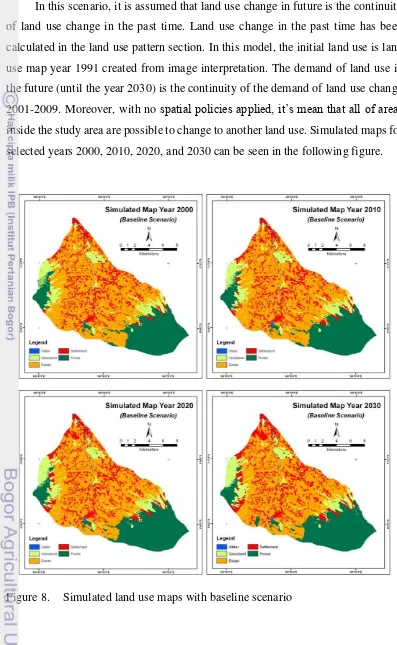
According to the change detection for the land use classification year 1991, simulated year 2000, year 2010, year 2020 and year 2030, it can be seen that settlement, forest and grassland area are increasing over time, whereas estate tend to decrease and water remains constant. Based on the findings, settlement area were significantly increase during the period 1991-2009 and causing the pressures in the study area.
Developing a model basin is an important step to assess the impact of land use changes on water yield in Upstream Cisadane Watershed using HEC-HMS. A configuration needs to be developed in the model basin to describe physical representation of a watershed based on its hydrology elements. In this research, there are seven hydrology elements available in HEC-HMS; Sub-basin, Reach, Reservoir, Junction, Diversion, Source, and Sink. The research employs 19 sub-basins, 9 reach, 9 junctions, and 1 outlet. Developing a model basin also includes calculation in 4 main sub-models, i.e.: loss model, transform model, base flow model, and routing model.
The model calibration done by adjusting the initial abstraction, curve number and impervious area values, until the results matched the field data. The process was completed manually by repeatedly adjusting the parameters, computing, and inspecting the goodness of fit between the computed and observed hydrographs. During calibration process by using half-year daily data (February 1, 2010 – July 31, 2010), the accuracy achieved 0.524 of R2. Performance of the model was objectively evaluated by using Nash-Sutcliffe Efficiency (NSE) and Relative Volume Error (RVE), in which it gave good efficiency value (NSE) of 0.67 and 42.9 % of RVE. By using three tests it can be stated that the model is satisfactory accepted.
Four hydrographs were simulated by using the same parameters in which was used during calibration and validation model. In this research, again the rainfall data of 2010 (February 1, 2010 – July 31, 2010 Period) was used as meteorological input. All these four scenarios were run using same parameters, except the curve numbers, percent impervious and initial abstraction are based on those previous land use condition. The simulated hydrograph obtain the peak flow and water yield information for four different land use scenarios. The values of each scenario peak flow are 81.00 m3/s, 81.10 m3/s, 81.00 and 81.10 m3/s for scenario 1, scenario 2, scenario 3 and scenario 4 respectively. While the value of water yield are 276,085.00 m3, 278,038.90 m3, 275,143.20 m3 and 279,178.20 m3 (all values for water yield are multiplied by 1000), for scenario 1, scenario 2, scenario 3 and scenario 4 respectively.
Copyright © 2014, Bogor Agriculture University Copyright are protected by law,
1. It is prohibited to cite in part or the whole contents of this thesis without referring to and mentioning the sources:
a. Citation only permitted for education purpose, research, scientific writing, report writing, critical writing or reviewing scientific problem.
b. Citation does not inflict the name and honor of Bogor Agricultural University.
FORECASTING LAND USE CHANGE AND THE IMPACT
ON WATER YIELD AT WATERSHED SCALE
YUSUF RAHADIAN
Thesis is a prerequisite to obtain degree Master of Science in Information Technology for Natural Resources Management Program Study
GRADUATE SCHOOL
BOGOR AGRICULTURAL UNIVERSITY B O G O R
Research Title : Forecasting Land Use Change and the Impact on Water Yield at Watershed Scale
Student Name : Yusuf Rahadian
Student ID : G 051 090 061
Study Program : Master of Science in Information Technology for Natural Resources Management
Approved by, Advisory Board
Dr. Ir. Suria Darma Tarigan, M.Sc.
Supervisor
Dr. Ibnu Sofian, M.Eng.
Co-Supervisor
Endorsed by,
Program Coordinator
Dr. Ir. Hartrisari Hardjomidjojo, DEA.
Dean of Graduate School
Dr. Ir. Dahrul Syah, MSc.Agr.
Date of Examination: December 12rd, 2013
ACKNOWLEDGMENT
Alhamdulillahirabbil’alamin, first of all, I would like to express my gratitude to Allah SWT., which by Allah SWT. helps, I can finally complete this study. Also, I
am indebted to many individuals during the course of study, I would like to thank
them through this opportunity:
To my extraordinary supervisor: Dr. Ir. Suria Darma Tarigan, M.Sc. for his
patience during the length of my research and my thesis writing. He has
provided me with guidance and motivation to develop and complete this
thesis. Dr. Ibnu Sofian, M.Eng., who has been so helpful and has provided
me with important guides and give me inspiration for writing my thesis into
its form now. I couldn’t have wished for better supervisors than those two. To MIT coordinator, lecturers, and MIT secretariat that has provided me with
opportunity to complete my study in Information Technology for Natural
Resources Management Study Program in a given time frame.
To my friends: Iwan Ridwansyah, M.Sc., Budi Nugroho, M.Sc., Triyanto,
M.Si., They are my partners that have provided me with invaluable support
through my study. Also thanks to Aswin Rahadian that has been there to share
his knowledge with me in mapping.
To my parents: Ani Rochaeni, Didi Achmadi, Tuti Trihatmi, and Edris; to my
brothers and sisters; Andina, Uci, Ismi, Andi and Taufiq, thanks for the
endless support, patience and prayers that have helped me through this study. Finally, to my wife, Dian Ekowati thank you so much for the love and support.
You taught me how to believe that I am capable. To my two amazing children,
Fathimah Azzahra and Umar Gandhi, I couldn't be more grateful to get to be
your father. I've learned so much from each of you.
I wish that this thesis will give positive contribution to all peoples who read it.
CURRICULUM VITAE
Yusuf Rahadian was born in Bandung, West Java, Indonesia on April 28th,
1981, studied Information Technology for Natural Resources Management with
specialization in Geographic Information System and Modelling. He attended
Forestry Management Study Program, Faculty of Forestry, Bogor Agricultural
University during 2000-2005 for his bachelor degree. He has been working with
several institutions e.g. Environmental Service Program of USAID Program, AidEnvironment Asia, and also have been working as independent consultant for
several projects in Forestry Management related issue, policy and the use of
Geographical Information System. Yusuf is currently working as an independent
CHAPTER I INTRODUCTION
1.1. Research Background
Increased use of natural resources as an impact of population growth and
economic development, conflict of interest, and the absence of coordination
between sectors/between areas (upstream, midstream, downstream) especially after
decentralization era have worsened the damage in watershed area. It is presented by
the higher occurrence of natural disaster e.g.: flood, landslide, and drought. Thus, since the last 30 years, the number of prioritized watershed in Indonesia is
increasing. One of them is Cisadane Watershed that based on Forestry Minister
Decree No. SK.328/Menhut-II/2009 is designated as one among 108 priority
watershed in Indonesia.
Many forms of nature changes in Cisadane Watershed indicate the occurrence
of natural resource degradation in its area. The width of Cisadane forest area is only
18.34%, far below the ideal number: 30% of total watershed area. This is worsened
with illegal logging in forest area and forest land use change outside the area, i.e. in upstream area. To understand and describe the cause of natural resource
degradation in this area, several comprehensive approaches are needed; from
biophysical, social economic and community culture factors. The research on
relation of land use change on hydrological condition is one way to aim for the right
watershed rehabilitation direction, so that the efforts conducted are better planned
and predictable.
Cisadane watershed forest area is only 18.34% (28,098.79 ha) of its total area.
The land use commonly found in Cisadane Watershed is farming, both dry farming
and paddy field. Total area of dry farming and mixed dry farming in Cisadane
Watershed is 47,368.55 ha (30.92%), paddy field area is 29,499.34 (19.25%),
settlement area is 34,194.25 ha (22.32%), and the rest 4,485.68 ha (2.93%) is bushes
and open land. Analysis of land use change conducted by Balai Pengelolaan Daerah
Citarum-for 989.7 ha and paddy field Citarum-for 201.9 ha; while the area of settlement increased Citarum-for
2,345.50 ha in between 2000-2009. In line with that, those changes have affected
the hydrological condition of Cisadane Watershed.
Prasetyo and Setiawan (2006) estimate the deforestation in Halimun Salak
National Park which part of it is in the area of Cisadane Watershed (21,586.1 Ha/
25.68 %). Several causes are illegal logging, land occupation and forest fire. Those
causes are all usually related to the community, both communities who live in the
surrounding area of forest or inside the forest.
The use of water resources and the control over its destructive force can only
be performed at its optimum if there is an adequate quantity, quality and continuity
of water resources. Conservation of water resources is critical to maintain and
increase the availability of water. Technically, water resource conservation efforts
can be performed by controlling the surface flow, accommodate the runoff from the
rain, to absorb water as much as possible and soak it into the ground.
Due to the vital role that water plays in the ecosystem, forecasting its yield
for the next generation has become critical to plan and manage its use. One primary
factor causes changes in water resources is the constant evolution in land use.
Forecasting the spatial distribution of water yield requires hydrology modeling.
The changes of land use patterns generate many social and economic benefits.
However, they also come at a cost to the natural environment. One of the major
direct environmental impacts of development is the degradation of water resources
and water quality (USEPA, 2001). Conversion of agricultural, forest, grass, and
wetlands to urban areas usually comes with a vast increase in impervious surface,
which can alter the natural hydrologic condition within a watershed. Since people
started to live in settlements they have adapted the land use and their needs. The
original land use has been replaced by cities, farmlands, industrial sites, roads,
canals etc. Furthermore, land use change is an ongoing process (Goldewijk, 2004).
Geographic Information Systems (GIS) has increasingly become a valuable
management tool, providing an effective infrastructure for managing, analyzing,
and visualizing disparate datasets related to soils, topography, land-use, land cover,
hydrologic and/or land use models as a data pre/post-processor have simplified data
management activities by enabling the easy and efficient extraction of multiple
modeling parameters at the watershed scale (Putnam and Chan, 2001; Ogden et al.,
2001). The improvement of land use change models combined with developments
in hydrological models allows more realistic predictions of future hydrologic
system. A new modeling approach is evaluated for assessing the impact of the land
use changes by combining a forecasting land use change model (Conversion of
Land Use and its Effects at Small regional extent/CLUE-s) with a hydrology model
(HEC-HMS). The benefits of such linkages, when supported by a common GIS
platform, are that planners can examine the present and future impacts land-use
policies may have upon hydrologic response characteristics of a specific watershed.
1.2. Problem Definition
One of the most important issues in watershed management is the use of land,
especially in the upstream catchment area. Changes in land use in upstream
catchment area, will give a concrete impact on the downstream watershed. In the
effort to fulfill their ends meet, especially food, and shelter, people can encourage
land conversion. As a result of the land conversion, the Cisadane River condition
seems quite apprehensive in the last two decades. Environmental degradation in
Cisadane watershed in both the upstream and downstream has a heavy impact to
the availability of water resources in Cisadane River.
Related to this fact, an in-depth study on land use change in Upstream
Cisadane Watersheds and its dynamics need to be conducted. Particularly, the
impact of land use change on water yield.
1.3. Research Objectives
This research purpose is to forecast the future of land use changes and assess
the impact of the predicted land use changes on water yield in Upstream Cisadane
This aim will be reached through the following objectives:
1. To forecast future land use changes in the Upstream Cisadane Watershed
predicted by a land use change model (CLUE-S),
2. To assess the impact of the predicted land use changes on water yield using
hydrology model (HEC-HMS).
1.4. Research Question
The present study aims to answer the following questions in order to achieve
the above-mentioned objectives. Research question related to the objectives are:
1. What are the major trends of future land use change?
a. How has the land use in study area changed during the period of
1991-2000 and 1991-2000-2009?
b. What are the trends of land use change in study area during 1991-2009?
c. What are the underlying driving factors that influence the land use change
in study area?
d. Which are the most important driving factors?
2. How are the impacts of land use change to water yield in the future?
1.5. Scope, Limitation and Assumption of Research
This study is intended to integrate remote sensing and GIS for forecasting
land use change in Upstream Cisadane Watershed. And also assessing the impact
of land use changes to water yield at Upstream Cisadane Watershed is conducted
using hydrology model.
Scope, limitation and assumption of this research are:
1) Study area as a boundary of system in this research is Upstream Cisadane
Watershed, with Empang as the outlet of the Watershed.
2) This study is intended to integrate remote sensing and GIS for forecasting land
land use change to water yield at Upstream Cisadane Watershed by employing
hydrology model.
3) Based on the limitation of the CLUE-s Model, land use type only divided into
five types, i.e.: water, grassland, estate, settlement and forest.
4) In this research, hydrology model is only employed to explore the effect of land
use change to water yield, by comparing hydrograph for each land use. Thus,
modeling result will not be calibrated.
1.6. Time and Study Area of Research
This research was conducted from August 2011 until December 2012. The
time is allocated for collecting, preparing and processing data; and also making a
final report in MIT Laboratory, Bogor - West Java. Data collection process was
conducted in Upstream Cisadane Watershed – Bogor.
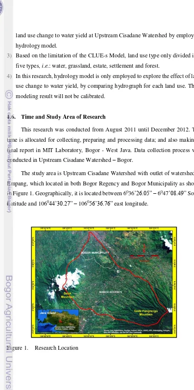
The study area is Upstream Cisadane Watershed with outlet of watershed in
Empang, which located in both Bogor Regency and Bogor Municipality as shown
in Figure 1. Geographically, it is located between 6036’26.05” – 6047’08.49” South
Latitude and 106044’30.27” – 106056’36.76” east longitude.
The water source of Upstream Cisadane Watershed is from Gunung Gede
Pangrango National Park and Halimun Salak National Park. Those river flows have
been used by the community around the river-banks to support and fulfill their daily
life needs, based on various kinds of practices. Based on its topography, Cisadane
Watershed upstream area is a hilly area with height to 3.000 masl and 40% slope.
Cisadane Watershed upstream area includes Bogor Regency and part of Bogor
District; its land use is dominated with forest, dry farming, estate, settlement and
open area.
1.7. Research Methodology in General.
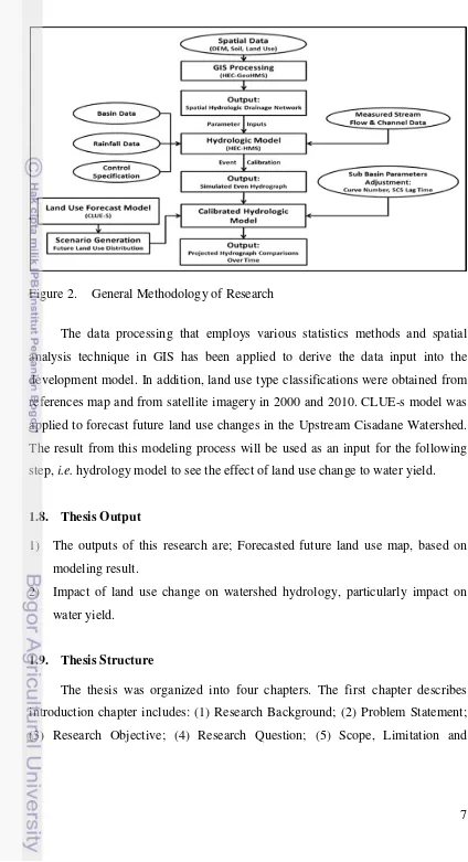
Research methodology in general for Forecasting Land Use Change and the
Impact on Water Yield at Watershed Scale is shown in Figure 2. Preparation of the
data into model input consists of spatial and non-spatial data. Spatial data can be
divided into raster and vector data. Topographical maps (Rupa Bumi Indonesia) that cover research area (including layers of administrative boundary, land use and road
network), village potential statistics map, geological map, forest maps, critical land
maps and soil map are used as vector data. Satellite imagery (ALOS-AVNIR)
imagery and SRTM-DTM were used as a raster data in this research. Statistical
data, including time series of population and village potential statistics of Bogor
Regency and Bogor Municipality area in 2000, and 2010 was used as non-spatial
Figure 2. General Methodology of Research
The data processing that employs various statistics methods and spatial
analysis technique in GIS has been applied to derive the data input into the
development model. In addition, land use type classifications were obtained from
references map and from satellite imagery in 2000 and 2010. CLUE-s model was
applied to forecast future land use changes in the Upstream Cisadane Watershed.
The result from this modeling process will be used as an input for the following
step, i.e. hydrology model to see the effect of land use change to water yield.
1.8. Thesis Output
1) The outputs of this research are; Forecasted future land use map, based on
modeling result.
2) Impact of land use change on watershed hydrology, particularly impact on
water yield.
1.9. Thesis Structure
The thesis was organized into four chapters. The first chapter describes
introduction chapter includes: (1) Research Background; (2) Problem Statement;
Assumption of Research; (6) Time and Study Area of Research; (7) Research
Methodology in General; (8) Thesis Output; and (9) Thesis Structure.
Generally, the result and analysis of this research activity are described in
chapter 2 and chapter 3. In the second chapter, analysis of land use change and its
driving forces will be discussed. Data processing that employs various spatial
analysis techniques and modeling in GIS has been applied to forecast the future
land use change. Meanwhile, chapter third describes the impact of the land use
change into water yield.
Finally, general conclusion and recommendation are drawn in chapter fourth
CHAPTER II
FORECASTING LAND USE CHANGE IN UPSTREAM CISADANE WATERSHED USING CLUE-S MODEL
2.1. Introduction 2.1.1. Background
Land use science can be defined as an inclusive, interdisciplinary subject that
focuses on material related to the nature of land use and land cover, their changes
over space and time, and the social, economic, cultural, political, decision-making,
environmental, and ecological processes that produce these patterns and changes
(Aspinall 2006). A variety of theories, methodologies, and technologies underpin
research on land use science, and, consequently, a number of basic and applied
science themes that are characteristic of land use research can be identified. These
reflect the interdisciplinary and integrated analysis required to comprehend land
use, as well as the role and importance of land use, land use change, and land
management and policy, and the importance of land use for sustainability (Raquez
et al. 2006). Land use is also considered a central part of the functioning of the Earth
system as well as reflecting human interactions with the environment at scales from
local to global.
Basic science questions in land use science include those that focus on (a)
dynamics of change in space and time; (b) integration and feedbacks between
landscape, climate, socioeconomic, and ecological systems (c) resilience,
vulnerability, and adaptability of coupled natural and human systems (d) scale
issues and (e) accuracy. Applied science addresses policy and management
questions in land use science including (a) addressing evolving public and private
land management issues and decisions; (b) interpretation and communication of
scientific knowledge for adaptive management of change in land use systems; and
(c) human and environmental responses to change (Aspinall and Hill 2008). The
applied issues also should be set against a need for explicit management of
participatory approaches. The need and role for spatially integrated dynamic models
of coupled natural and human systems in the contexts of study and management of
land use change underpin this discussion.
The rising awareness of the need for spatially explicit land-use models within
the Land-Use and Land-Cover Change research community (LUCC; Lambin et al.
2000a; Turner et al. 1995) has led to the development of a wide range of land-use
change models. Whereas most models were originally developed for deforestation
(Kaimowitz and Angelsen 1998; Lambin 1997) more recent efforts also address
other land use conversions such as urbanization and agricultural intensification
(Brown et al. 2000; Engelen et al. 1995; Hilferink and Rietveld 1999; Lambin et al.
2000b).
Spatially explicit approaches are often based on cellular automata that
simulate land use change as a function of land use in the neighborhood and a set of
user-specified relations with driving factors (Balzter et al. 1998; Candau 2000;
Engelen et al. 1995, Wu 1998). The specification of the neighborhood functions
and transition rules is done either based on the user’s expert knowledge, which can
be a problematic process due to a lack of quantitative understanding, or on empirical
relations between land use and driving factors (Pijanowski et al. 2000; Pontius et
al. 2000).
A probability surface, based on either logistic regression or neural network
analysis of historic conversions, is made for future conversions. Projections of
change are based on applying a cut-off value to this probability surface. Although
appropriate for short-term projections, if the trend in land-use change continues,
this methodology is incapable of projecting changes when the demands for different
land-use types change, leading to a discontinuation of the trends. Moreover, these
models are usually capable of simulating the conversion of one land-use type only
(e.g. deforestation) because they do not address competition between land-use types
explicitly.
The Conversion of Land Use and its Effects (CLUE) modeling framework
(Veldkamp and Fresco 1996, Verburg et al. 1999a) was developed to simulate
driving factors in combination with dynamic modeling. In contrast to most
empirical models, it is possible to simulate multiple land-use types simultaneously
through the dynamic simulation of competition between land-use types.
2.1.2. Objective
The objective of this study is to forecast future land use changes in the
Upstream Cisadane Watershed predicted by a land use change model (CLUE-s).
2.2. Literature Review
2.2.1. Forecasting Land Use Change
Several methods have been developed for forecasting land use change, with
varying degrees of sensitivity to the influence of transportation networks. The
simplest types of models for forecasting land use change are Markovian models
(Brown et al. 2000; Weng et al. 2002) such as Markov chain models, which tend to
treat land use change as a stochastic process. Assuming that rates of change between
land use types are more or less constant from one period to the next, Markovian
models project land use transitions forward to any given future date, eventually
reaching an equilibrium distribution of land uses. These models tend to have a
limited ability to incorporate transportation networks and other spatial features,
except as states (e.g., land use types) in the model. More often, they are applied to
analyses of land use change.
Cellular and agent-based models have recently gained greater acceptance as
tools for simulating land use change in urban areas. Advances in computational
power and data storage have facilitated the development of models that
disaggregate urban space to a greater degree and can operate with individuals or
land parcels as the units of analysis, rather than zones. These include
micro-simulation models of urban development, as well as models based on a cellular
automata framework (Jantz et al. 2005). Cellular automata models emphasize
neighbor effects and dynamic interactions between agents (with land use cells as
agents and attempt to simulate their behavior in terms of location and travel choices.
Micro-simulation models of land use are often coupled with transportation models
and are integrated into larger urban simulation models (Waddell and Ulfarsson
2003).
Despite these methodological advances, regression models continue to be a
popular method for modeling and simulating land use change. Indeed, many
simulation models with a land use component use regression methods, either in the
form of discrete models of land use change (Landis and Zhang 1998) or within
hedonic or bid-rent frameworks for land prices (Waddel 2003). Regression models
allow the identification of exogenous variables, which are thought to influence
patterns of development. The variables can represent physical and social influences
on development (Verburg 2004), neighborhood effects (Verburg 2004; Zhou and
Kockelman 2007), or the effects of transportation and accessibility. It is these latter
effects that are of the greatest interest in the current context. While regression
techniques have been used previously to identify the correlates of highway network
growth in terms of land use and population characteristics (Levinson 2007).
2.2.2. Modeling Land Use Change
The land-use change model, Conversion of Land-Use and its Effects at Small
regional extent (CLUE-S) (Verburg 1999), is used to simulate future land-use
change. The CLUE-S model is an empirical based model developed at the
University of Wageningen in the Netherlands. The model attempts to identify
causes of land use changes (driving forces), using a multivariate analysis on the
possible contributors, to empirically derive rates of change (Verburg et al. 1999).
The CLUE-S model has been chosen for the land-use modeling in this study
based on the selection criteria developed by the US Environmental Protection
Agency (US EPA, 2000). The most important reasons for choosing this model were:
the flexibility on the input data (driving forces), the possibility of linking the output
to another model (e.g. Hydrological Model/HEC-HMS model), and free access to
2.3. Methodology
Changes in land use pattern are related to a large number of biophysical and
socio-economic factors. The modeling of spatially explicit changes in land use
pattern requires, therefore, a large database of factors considered to be important in
the case study. Therefore, the database is not similar for every application. To run
the model it is minimally needed to have spatially explicit data for at least 1 year.
However, to allow calibration and validation model works, it is necessary to have
data of another different year. To meet this necessity, the research will employ data
from 2 different years, with 6 years’ time difference, i.e. 1991 and 2009.
2.3.1. Data Preparation
2.3.1.1. Data Requirement for Land Use Change Model
For the simulation of dynamics of the spatial pattern of different land use
types, data are needed for the land use distribution and a number of biophysical and
socio-economic parameters that are considered as important potential drivers of the
land use pattern. These drivers are most commonly variables that describe the
demography, soil, geology, climate and infrastructural situation. This study only
considers the biophysical aspects, while the socio-economic aspect is considered
constant (Business as usual).
The data required to analyze land use change process and build scenario
development were obtained from various sources. The data are derived from
multispectral satellite data, extracted from digital topographic data, and from spatial
processing of statistical data. According to type, data are divided in three: remotely
sensed data, digital topographic data and statistical data. How the data were
collected and used will be explained below.
Remotely Sensed Data
Remotely data used in this study comprises of Landsat images 1991 (30 m),
and ALOS-AVNIR image 2009 (10 m). These data will be used for land use change
analysis and input for trend extrapolation to calculate land use requirements year
Table 1. Remotely Sensed Data Requirement for Land Use Model
Image Resolution Date Acquisition Source of Data
Landsat TM 30 m 28 July 1991 GLOVIS
ALOS AVNIR 10 m 17 July 2009 BTIC – BIOTROP
Topographic data
Topographic data sets are obtained from Agency of National Survey and
Mapping (Bakosurtanal – Geospatial Information Agency/BIG, nowadays), Bogor.
These data are digitized from topographic map scale 1:25.000 and are extracted for
selected layers, including road, facilities and public service distribution, and central
of economic. All layer data have been digitalized, infrastructure and facilities, road,
river, public services and industries location. Data sets used in this study can be
seen in the following table.
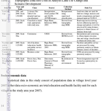
Table 2. Topographic Data Sets Used in Analysis Land Use Change and Scenario Development
Land uses data are used for land use change analysis and change and pattern, it will be processed by using distance
Continuous USGS Derived from SRTM-Level 2 be used as spatial policy in the model.
Socio-economic data
Statistical data in this study consist of population data in village level year
2007. Other data socio-economic are total education and health facility unit for each
Table 3. Statistical data used in analysis land use change and scenario development
Data Year Source Description Data Use Population 2007 Village potential
statistic –
In order to enable analysis and modeling in the CLUE modeling framework
the data need to be converted into a consistent format. Therefore the data are
converted to raster format. Grid size depends on the scale and resolution of the
original data. All grids should have the same (equal area) projection and be
geo-referenced with exactly the same extent and cell size.
All data are communicated with the CLUE-S model through ASCII files,
meaning that the data are stored in a text file that contains all values of the individual
grids, presenting the values for separate cells. In this format the values for the
individual cells are stored in rows and columns with a header that describes the
format, like number of columns and rows and the coordinates of the upstream left
corner. Data can also be stored in one single column containing all the cells.
2.3.1.3. Data Normalization
The maps used as independent variables are created in raster format. To
produce these maps, vector data are transformed into raster format with a spatial
resolution of 50 m. This spatial resolution is appropriate with image data, which
also have a resolution 50 m.
To balance the range of data values, all of variables are normalized into 0 –
1. Normalization is done by dividing the value of each grid cell with the highest
value of cell data to achieve similar data range. This method is important because
of the sensitivity of data transformation in logistic regression. Moreover, in the
multivariate analysis such as logistic regression, the continuous independent
2.3.2. Land Use Scenario Development by using CLUE-S Model
A development scenario of land utilization in this study is addressed to
understand the dynamic of land use change. Method to implement land use
scenarios in this study is based on CLUE-S model (Veldkamp, et al., 1996), which
emphasizes on how scenarios can be demonstrated in study area by using simulation
of land use change.
CLUE-S model is chosen in this study because of its adaptability to local scale
and successful applications in tropical regions that make it appropriates to be
applied in study area. Besides that, this model is based on an analysis of the spatial
structure of land use that it makes the model is not bounded by the behavior of
individuals or sectors of the economy. In the other hands, CLUE-S model provides
many opportunities to include actor-behaviors and feedbacks from policy makers.
The possibility to simulate different scenarios for various land use types at the same
time makes the model powerful to support land use analysis in study area.
2.3.3.1. Land Use Classification
Land use maps are derived from classification of Landsat TM images year
1991, and ALOS-AVNIR images year 2009. In this study, the images are classified
in five classes based on land use condition in the area.
Table 4. Land use classification in study area
Land Use Code Description
Water 0 River, lake
Grassland 1 Shrub, bare land
Estate 2 Irrigated & rain fed paddy field, dry land Settlement 3 Residential area, developed area
Forest 4 Forest, no matter inside or outside forest area
2.3.3.2. Location Characteristics
Location characteristics are a set of factors that affecting land use changes.
The combination of factors provides preference for a specific type of land use to
between land use and driving factors is calculated by using logistic regression. The
results of regression analysis are used to create probability map for each land use
type. The driving factors used in this study can be seen in Table 5.
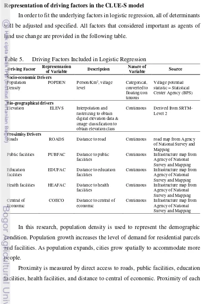
Representation of driving factors in the CLUE-S model
In order to fit the underlying factors in logistic regression, all of determinants
will be adjusted and specified. All factors that considered important as agents of
land use change are provided in the following table.
Table 5. Driving Factors Included in Logistic Regression
Driving Factor Representation
POPDEN Person/Km2, village
level
Elevation ELEVS Interpolation and
rasterizing to obtain
Roads ROADS Distance to road Continuous road map from Agency
of National Survey and Mapping
Public facilities PUBFAC Distance to public facilities Health facilities HEAFAC Distance to health
facilities
COECO Distance to central of economic
Continuous Infrastructure map from Agency of National Survey and Mapping
In this research, population density is used to represent the demographic
condition. Population growth increases the level of demand for residential parcels
and facilities. As population expands, cities grow spatially to accommodate more
people.
Proximity is measured by direct access to roads, public facilities, education
cell is mainly measured with straight-line distance to the specific location, where
the straight-line is measured by using Euclidean distance to the target location.
It is predicted that proximity factors become more dominant in this study,
because of relatively smooth topography of the study area. Distance to facilities,
and distance to road become important determinants in predicting land use change.
Furthermore, elevation data is considered important in this area, although it has
little variation. Elevation is significant for estate and settlement land use area, where
it is associated with the distribution of irrigation water to agricultural crops and
landscape for residential area.
Another fact is that the density of population is measured by the relative
density, not an absolute density. Density is calculated based on the number
population (person) divided by the village area (Km2). This is not a best-fit method
to measure the density where density should be measured in urban area or named
absolute density. However, the calculation of the absolute density of urban areas
land use cannot be applied to logistic regression, because it will produce data that
are bias, where the regression calculation applied to the same extent of areas.
2.3.3.3. Statistical Analysis
Logistic regression is divided in two types, including binomial and
multinomial regression. Binomial regression, which is employed in the research,
uses dichotomous value in the dependent variable, whereas the type of independent
variable could be categorical or continuous. In land use analysis, logistic regression
is used to examine the relation between land use and possible driving factors. The
results of this analysis are coefficient values that show the contribution of each
driving factor to land use change. The formula is:
� − = � + � � + � � + ⋯ + ���� (Verburg 2002).
Where : is the land use change probability
��… are independent factors
To achieve the validity of land use change estimation, the model should be
supported by the procedure to identify the driving factors that are statistically
independent and to determine the significance of driving factors. One of methods
to identify the driving factors that have significant contribution to land use pattern
is the stepwise procedure. In the stepwise procedure, all of driving factors are
involved in one step and eliminated according to their significance values. A driving
factor that has a lower value than the significant threshold will be excluded from
the analysis. In forward procedure, the analysis starts with one factor and continues
to other factors respectively.
ROC (Relative Operating Characteristics) is a method to measure the
goodness of the statistical model. The probability of each land use resulted from
logistic regression is compared to the real land use map to calculate the equal
category of each grid cell between those maps. According to Pontius and Schneider
(2001), this method will depict the capability of regression equation to represent
land use characteristics. The range of ROC value is between 0 – 1, where ROC
value below 0,5 is categorized in low or completely random, 0,5 – 0,6 is good, 0,6
– 0.99 is very good and 1.0 is fit/perfect. The goodness of the logistic regression equation to represent land use condition indicates the suitability of driving factors
as determinant of land use change.
2.3.3.4. Land Use Type Specific Conversion
Conversion setting for specific land use type is addressed to determine the
temporal dynamic of the simulation by using reversibility of land use changes. This
method will be implemented by using three different decision rules that represent
the situation of study area:
1. Some land use types are unlikely to be converted into another land use type
after first conversion.
2. Other land use types are converted more easily. Forest and grassland are more
likely to be converted into another land-use type soon after their initial
3. Other remains land use types operate in between those settings, where the
conversion will occur in specific condition. An example is grassland will be
converted to estate area if estate area is more profitable.
Table 6. Land use conversion matrix for study area
Land Use Future
1 likely to conversion; 0 unlikely to conversion
This method is one of specific setting to determine temporal dynamic of land
use simulation. Land use with high investment will not easily be converted to other
uses. Moreover, because of the differences of conversion behavior, dimensionless
factor is added to each land use type. This factor represents elasticity conversion,
ranging from 0 (easy conversion) to 1 (irreversible change). Water area and
settlement area is an example of this rule, where the elasticity value for urban built
up area is set 1 that shows urban built up area is hard to be converted to another
type of land use. Grassland and forest area are more easily to be converted and the
value is 0.4. Estate is set to more difficult to be converted, so the elasticity value is
0.6. The justification of the elasticity values of land uses in this study is based on
field observation and local knowledge and adjustment for the model. The range of
values can be seen in following table.
Table 7. Settings of conversion elasticity in the study area
Land Use Type Conversion Elasticity
2.3.3.5. Scenario Setting
The scenarios presented are not necessary the most realistic, but are made in
such a way that they provide information on the functioning of the model. A
scenario for the CLUE-S model consists of a file with land requirements and a file
that indicates areas where restrictions to conversion apply.
Land Requirements
Land use requirement (demand) is calculated for every land use in the whole
of study area. This requirement becomes a constraint of area needed for simulation.
Demand of land use will be specified in every year by using extrapolation of past
land use change trends that have been quantified before (year 2001-2009).
Future land utilizations are based on two considerations:
1. Baseline.
Population growth is assumed stable and land requirements of 2009-2020 keep
linear change based on the trend in the period 2001-2009. According to the
baseline scenario, the demand of land use year 2009-2020 will be extrapolated
from the annual change in the period 2001-2009.
2. The increasing growth of population.
The assumption is based on a slow growth of population in study area that has
effects on increasing of demand of settlement and estate land use. In this
scenario, the demand of urban built-up area is assumed increased twice from
the demand of urban built-up area in baseline scenario.
Spatial Policies
Spatial policies (restriction) can influence the pattern of land use change.
Spatial policies mostly indicate areas where land use changes are restricted through
policies. Besides that, spatial policies can imply stimulation arrangements for a
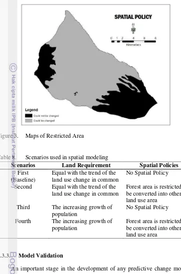
certain land use on a location. In this study, forest designation map is used as area
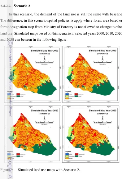
Figure 3. Maps of Restricted Area
Table 8. Scenarios used in spatial modeling
Scenarios Land Requirement Spatial Policies
First (Baseline)
Equal with the trend of the land use change in common
No Spatial Policy
Second Equal with the trend of the land use change in common
Forest area is restricted to be converted into other land use area
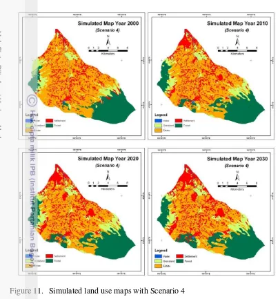
Third The increasing growth of population
No Spatial Policy
Fourth The increasing growth of population
Forest area is restricted to be converted into other land use area
2.3.3. Model Validation
An important stage in the development of any predictive change model is
validation. Typically, one gauge means the understanding of the process and the
power of the model by using it to predict some periods of time when the land use
conditions are known. This is then used as a test for validation.
The first is called ‘validate’, and it provides a comparative analysis on the
basis of the Kappa Index Analysis. Kappa is essentially a statement of proportional
= � ∑� − ∑��= ���− ∑��=� ��+ , �+�
�+ , �+�
� �=
Where : � = Total number of sites in the matrix,
� = Number of rows in the matrix
��� = Number in row i and column i
��+ = Total for row i, and
�+� = Total for column i.
Kappa can be used to determine if the values contained in an error matrix
represent a result significantly better than random (Jensen 1996).
2.4. Result & Discussion
This section will mainly discuss the results of overall analysis, including
analysis of land use changes, examination of driving factors in logistic regression
and land use scenario development by using relevant variables in the CLUE-S
model. The first section explains the result of identifying, quantifying and trend
analysis of land use change. The second section of this chapter mainly demonstrates
the use of relevant variables logistic regression analysis in development scenarios
of future land use. The model used will depict the effect of land use change to the
future land use. All of sections of this chapter will be directly followed by
discussion to provide clear explanation about all of the findings of this research.
2.4.1. Land Use Pattern
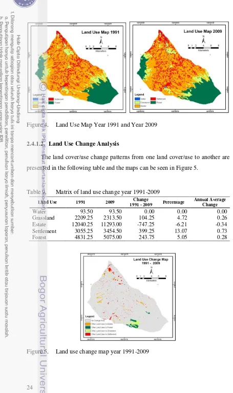
2.4.1.1. Land Use Maps Year 1991 and 2009
According to the classification processes, there are five land uses that could
be identified from all of images: water, grassland, estate, settlement and forest.
Description of each land uses are explained in Table 4 and the location and
Figure 4. Land Use Map Year 1991 and Year 2009
2.4.1.2. Land Use Change Analysis
The land cover/use change patterns from one land cover/use to another are
presented in the following table and the maps can be seen in Figure 5.
Table 9. Matrix of land use change year 1991-2009
Land Use 1991 2009 Change
1991 - 2009 Percentage
Annual Average Change
Water 93.50 93.50 0.00 0.00 0.00
Grassland 2209.25 2313.50 104.25 4.72 0.26
Estate 12040.25 11293.00 -747.25 -6.21 -0.34
Settlement 3055.25 3454.50 399.25 13.07 0.73
Forest 4831.25 5075.00 243.75 5.05 0.28
Based on the findings about land use changes in year 1991 and 2009 above,
it can be noted that urban settlement area experienced the most significant
development followed by forest and grassland. However estates tend to decrease
and river is stable during the 1991-2009 period.
2.4.1.3. The Trends of Land Use Change during 1991-2009
According to the change detection for the land use classification year 1991
and 2009, it can be seen that settlement, forest and grassland area are increasing
over time, whereas estate tend to decrease and river remains constant. The trends
of land use changes of the area during 1991-2009 are presented in following figure.
Figure 6. Trends of land use change year 1991-2009
2.4.2. Analysis of driving factors of land use changes 2.4.2.1. Logistic regression results
The results of logistic regression between land use and independent variables
are presented in this section. Each land use has independent variables or driving
factors that influence to its pattern. In logistic regression analysis, five classes of
land use are included in the regression calculation.
The selection of the significant and non-significant independent variables is
based on a enter procedure (see 2.3.3.3.). The variables, which have coefficient
variables above 0.02 will be classified as non-significant and automatically
removed in the calculation process. All of significant variables are automatically
selected in the results of enter procedure and will be used in the calculation of land
use probability. Practically, enter procedure in logistic regression is done by putting
all independent variable in the process at the same time in the iteration process. The
result can be seen in the Table 10.
Table 10. Results of logistic regression between land use pattern and driving factors
Variable Water Grassland Estate Settlement Forest
Total number of
Enter procedure; Significant at: < 0.01 entry level and > 0.02 removal
*) Has significant value above 0.02 (See Appendix 5.); ** Not statistically significant (value above 0.02)
2.4.2.2. Logistic regression interpretation
The number of driving factors used in this regression analysis is 7 variables.
Each driving factor has a different effect on every type of land use. The effect of
each driving factor is indicated by the coefficient β in logistic regression result,
which presents how much variance from the use of land that can be explained by
the driving factors. A large positive β value indicates a strong positive relationship between the independent and dependent variable (land use change), while a large
negative β value indicates a strong negative correlation with land use change.
Besides the effect of driving factors, the results of logistic regression can be
used to indicate which driving factor that has the biggest influence to the land use
change. How big the influence of each driving factor is indicated in exponential β
exponential β for settlement area (Table 10.), it can be interpreted that population density has the biggest influence to the land use change in the area compared to the
other driving factors. As an example of interpretation, population density has
coefficient β value 1.081and exponential β value 2.948, which means the increase of 1 unit of population density, will influence 1.081 unit of settlement area to change
with the probability value 2.948. In the other words, 1 unit influence of population
density has 2.948 probability of settlement area to change. This interpretation also
applies to other driving factors and other land use types involved in the logistic
regression model.
According to the stepwise procedure in the logistic regression for forest area
(Table 10.), some variables have significant values, including population density
(POPDEN), elevation (ELEVS) distance to main road (ROADS), distance to public
facility (PUBFAC), and distance to education facility (EDUFAC). In the other
hand, distance to health facility (HEAFAC) and distance to center of economy
(COECO) have non-significant values and removed from the calculation process.
In general, the result of logistic regression for forest area is appropriate with the
pattern of land use change. In other case for water (Appendix 5.), population
density, elevation, distance to main roads, distance to health facility, and distance
to central of economy have significant values. In the other hand, distance to public
facility and distance to education facility have non-significant value. The interesting
in this case is constant for the water case has non-significant value (0.04), that’s
mean the equation for water automatically removed in the calculation process, when
it is inserted in the model, the probability of river will not change from year to year.
It same with the assumption that water area will not change during the model run.
Regarding to the relationship in settlement case, it can be seen that population
density, and distance to health facility have positive effects to the urban built-up
area. In other hand, elevation, distance to main roads, distance to public facility,
distance to education facility and distance to center of economic have negative
effect to the probability of settlement area to change. The relationship of each
driving factor with settlement area change in this research is reasonable for the
from the existing settlement, while distance to main roads, public facility, education
facility and center or economy, are far away from settlement area.
Based on the value of the coefficients of these driving factors, the regression
equation can be created to indicate the influence of the driving factors and the
overall probability for each land use change. By using ROC, the probability of each
land use is evaluated and compared to the existing land use. The comparison is
based on the number of cells that equal between the maps. The percentage of ROC
shows how the regression equation can be used to predict the future land use change
based on its probability.
According to the results, the values of ROC for probability of water area,
grassland area, estate area, settlement area and forest area are 0.903, 0.701, 0.780
and 0.813 and 0.994 respectively. Based on some literatures, these values are
categorized as better (very good). These results are valid, which is confirmed to the
results of some similar studies using logistic regression, including Hu and Lo (2007)
and Verburg et. al. (2002). The differences are on the direction of the relationship
and the most influenced driving factors and land use as explained before. Moreover,
this result is reasonable because the influence of driving factors depends on the
location and the situation where the model is applied (Xie et al, 2009).
After measuring the goodness of the logistic regression results for every land
use type, it can be concluded that the model capable to represent the land use
changes within the Upstream Cisadane. However there are some considerations that
should be reviewed related to data adequately, data quality, and scale of analysis.
The availability of relevant data should placed is the most important consideration
because it reflect dynamic of the area being modeled (Verburg et al, 2004). The
socio-economic data such as preference of society to choose new settlement
location with lower price are not used in this research because of unavailability of
data. As these data could improve the understanding of complex land use behavior,
their availability should be incorporated in further research.
Scale of analysis is another important issue to be discussed because this
research is conducted by using images that have middle scale resolution (50m x
(Verburg et al, 2002), it has possibility to be improved with higher spatial resolution
data to acquire more detailed information about Upstream Cisadane behaviors. The
more information could be derived from the data, the more understanding about
land use dynamic in the location (Cheng, 2003). However, it should be noted that
data with large resolution need more capacity for iteration process and when it is
combined with the land use model, the capacity data could excess the processing
capability of the model.
Furthermore, this research indicates that logistic regression analysis is very
sensitive in multistage analysis such as data transformation and spatial sampling.
According to Cheng (2003), the logarithmic data transformation and the
combination of sampling type could significantly influence the parameter
estimation and model accuracy. Related to sampling method, this research has
employed appropriate sampling method. The method has been discussed in the
conceptual model section, where all of independent variables are normalized to the
range 0-1 to create similar range of data and avoid different data dimension. This
method is valuable to overcome the sensitivity of logistic regression calculation to
the various variables and the result is more reliable in examining the influence of
driving factors of land use change.
According to the findings and their interpretation above, the conclusion can
be drawn about the usability of statistical analysis by using logistic regression to
examine the relationship between driving factors and land use change in study area.
The results give evidence about the influence of each driving factor on each land
use type, the magnitude of its effect and the most influencing driving factors for
each land use type. Regardless the limitation in data, the method used and the results
are satisfactory because they capable to reveal the relationships that were not known
before and provide new insight about land use behavior in the area, such as the
growth of residential area in the adjacent of secondary road and at a specific
distance from primary road. Moreover, the combination between logistic regression
and CLUE-S framework becomes the solution for the limitation of logistic
regression model where it can only be used to predict the location of land use
Based on these reasons, logistic regression model in this research is combined with
CLUE-S framework to predict future land use change in the area.
2.4.2.3. Land use probability maps based on logistic regression
The final results of the logistic regression model are used to create probability
map of each land use, including urban built-up area, agricultural area, mix
vegetation, ponds area and river. The value of probability of each land use type is
in the range between 0 and 1. The probability maps can be seen in Appendix 7,
which show that the darker of the color, have the higher the probability of land use
to change. The range of probability water area is 0.870 – 0.984, grassland area is 0
– 0.273, estate is 0 – 0.929, settlement is constant is 0.5, and forest area is 0.002 – 0.966. The interesting from probability of settlement where the constant is 0.5,
that’s mean every pixel in a whole study area has the same probability to change to
settlement (see Appendix 7).
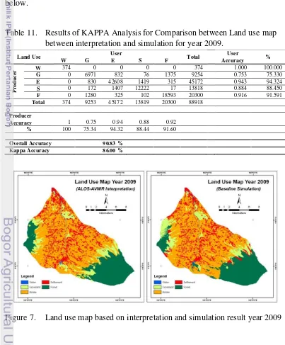
2.4.2.4. Model Validation
In order to achieve a valid land use simulation, the validity of this model is
examined by using the observed land use map year 2009, which has been created
from image interpretation. Land use map year 2009 resulted from the simulation is
compared to the observed land use map year 2009 to measure the number of equal
grid cells in both of maps and the similarity of land use pattern. Similar with the
method done by Zhu et. al. (2009), this approach results a overall accuracy which
indicate the degree of similarity between those two maps and Kappa accuracy that
depicts the degree of pattern similarity. According to Landis and Koch (1977),
Kappa accuracy is useful to calculate the agreement of two maps. It is stated that
Kappa values > 80% is categorized as fit, 60% – 80% is high agreement, 40% –
60% is moderate and <40% is poor. Therefore Kappa accuracy is used in this
research to measure pattern similarity.
After comparing both maps, the results show that overall accuracy and Kappa
pattern in study area and it can be used to predict future land use pattern.
Furthermore, related to the uncertainty of land use pattern in the future, 90.83 %
overall accuracy and 86.00 % Kappa accuracy values show that all of driving factors
capable to reduce the uncertainty because they capable to describe the land use
behavior that will shape the future land use condition. The results are confirmed to
the statement of Pontius and Neeti (2009) where high agreement resulted from
validation process indicates that the processes of land use change during the
calculation are stable trough the interval of validation and suitable to be used in
simulation process. The result of Kappa measurement can be seen in the table
below.
Table 11. Results of KAPPA Analysis for Comparison between Land use map between interpretation and simulation for year 2009.
Land Use User Total Accuracy User %