Computing Scalar Variance
Colleen M. Kaul1
, Venkat Raman1
, Guillaume Balarac2
and Heinz Pitsch3
1
Dept. of Aerospace Engineering and Engineering Mechanics, The University of Texas at Austin, Austin, TX 78712, [email protected],
2
MOST/LEGI, BP53, 38041, Grenoble Cedex 09, France
3
Center for Turbulence Research, Stanford University, Stanford, CA 94305, USA
Summary. The results of a novel procedure fora posteriori testing show that the predictions of a dynamic model for the subfilter variance are sensitive to accumu-lated errors in the evolution of the filtered scalar field as well as to numerical errors incurred in evaluating the variance model at a single time step. Tests were performed on homogeneous, isotropic filtered scalar fields simulated using exact and modified wavenumbers corresponding to second, fourth, and sixth order accurate finite dif-ference schemes. The sixth order scheme showed close agreement with the spectral method in terms of the distribution of predicted subfilter variance values, which were assessed using nonparametric techniques. The second order scheme produced, on average, substantially higher values of subfilter variance. Valid methods for com-paring models were sought that account for the variability of statistical estimates made from a spatially correlated sample, and some preliminary approaches were presented.
Key words: subfilter scalar variance, nonparametric statistics, subfilter model er-ror analysis
1 Introduction
In conserved scalar methods for large eddy simulation of non-premixed com-bustion, the subfilter scalar variance indicates the degree of small-scale mixing. The subfilter variability of scalar values is approximated by a beta distribu-tion, which is fully specified by the values of the filtered scalar and subfilter scalar variance. However, the subfilter variance, defined asZ′2
=Z2
−Z2, must itself be modeled. A common modeling approach uses an algebraic relation of the form Z′2
=C∆2
pro-cess, small errors in variance estimation can lead to large errors in species concentrations.
Because of the gradient-squared dependency of the dynamic model, it has been inferred that finite difference methods result in underestimation of the variance in actual simulations using grid-based filtering. However, DNS-based a priori tests [5] have indicated that this explanation is too simplistic. In fact, finite difference implementation of the dynamic procedure resulted in overestimation of the model coefficient, partially canceling the numerical un-derprediction of the gradient-squared quantity. While such static tests on DNS data are useful in isolating specific sources of error in subfilter variance esti-mation, they are not necessarily indicative of the errors encountered in LES simulations because they do not account for the interaction of the variance model with an LES-evolved filtered scalar field. Initial results suggest that the effect of errors in the filtered scalar evolution on subfilter variance pre-diction is significant relative to effects due solely to subfilter variance model implementation [6].
A second reason whya priori tests may lack extensibility to LES results is that a DNS field provides only one sample of the small scale turbulence that could correspond to a given filtered field. Generally, however, interest is focused on estimating one-point statistics rather than the statistics of the field per se, and spatial averages over homogeneous directions are used in place of ensemble averages. Most methods for estimating one-point statistics assume independent and identically distributed data. While the latter criterion is usu-ally satisfied , the former cannot be. Both real and simulated turbulence fields, obviously, exhibit correlation in space and time. If methods based on indepen-dent samples are applied to correlated data, it should be with the awareness that the effective sample size is significantly reduced. With a smaller sample, it becomes more important to distinguish between sample estimates and the actual population value of a statistic and to provide some quantification of the uncertainty of the estimate. This is a point that has been largely neglected in a priori tests of subfilter models.
2 Details of LES Computations
To study the effect of numerical error in scalar evolution on subfilter variance prediction, we have formulated a novela posterioricomputational experiment. A pseudospectral code for simulation of homogeneous isotropic turbulence was modified to solve a governing equation for the filtered scalar field with exact and modified wavenumbers. A computational domain of 2563
of 8η and 16η were considered, where η is the Kolmogorov length. Filtered velocities were supplied by explicit filtering of a DNS velocity field, which was forced at the large scales to maintain Reλ = 80. The initial conditions for
all filtered scalar evolutions were obtained by filtering the initial conditions of a DNS-resolution scalar with Sc = 1. All scalar fields were decaying, and simulations were carried out over a period of about one eddy turn-over time,
τ, as calculated from the DNS velocity field.
Two analytically equivalent forms of the filtered scalar transport equation were considered, as the accuracy of the diffusion operator in finite difference implementations of the equation has been recently noted as an important factor in the prediction of subfilter variance [6]. The filtered scalar transport equation is frequently solved in the form
∂Z
which will be referred to as the conventional formulation. However, second derivative terms are approximated more accurately by a single application of a second derivative scheme than by two applications of a first derivative scheme. This suggests that Eq. 1 be written in a modified formulation as
∂Z
Modified wavenumbers for lower order finite difference schemes deviate significantly from the ideal value, causing the diffusion operator to be less effective at small scales [7]. Higher order schemes possess modified wavenum-bers that are close to the ideal value for a larger portion of the spectrum, thereby increasing accuracy. The form of the diffusion term in Eq. 2 is mo-tivated by the fact that the modified wavenumber-squared representation of a second derivative scheme is more accurate at high wavenumbers than the square of the modified wavenumber of a first derivative scheme of the same nominal order of accuracy.
A recently developed dynamic subfilter variance model [1] was imple-mented for each scalar with the same scheme used to solve its transport equation. This model, like its predecessor [9], calculates an averaged model co-efficient over homogeneous directions according toC =#LM$/#MM$where
#·$ indicates a volume average in the present context. The quantitiesL and
M are calculated at the level of a test filter, ∆. The Leonard term has#
the form L = Z$2−Z#
2
, while the model’s gradient-based term is given by
M=∆#∇Z# · ∇Z#.
distributions of subfilter variance values. Since there is no evidence for a para-metric form of the distribution, non-parapara-metric approaches, accounting for the correlation of the data, are necessary. Details of the methods are provided below.
3 Results
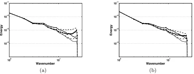
Fig. 1 compares spectra of filtered scalar fields att= 0.7τ to assess the effects of errors in the diffusion operator. Comparison with the filtered DNS scalar spectrum indicates that the subfilter flux model is too diffusive when imple-mented exactly, as in the spectral LES solution. For reference, simulations were also performed using the exact convection operator and their spectra computed. Convective term errors most noticeably affect the middle range of wavenumbers, especially for the second order scheme, while errors in the diffusive term are manifested at the highest wavenumbers as an accumulation of energy. Lack of diffusion at these scales is apparent even when an exact convective operator is used, albeit less severe. The modified diffusion term in Eq. 2 clearly is more effective at removing small scale energy.
All results presented below are for scalar fields evolved using the same scheme for convection and diffusion operators. We next examine the extent to which the subfilter variance field is spatially correlated and how the degree of correlation is affected by the choice of filter width and numerical scheme.
100 101 10−4
10−3 10−2 10−1
Wavenumber
Energy
(a)
100 101
10−4 10−3 10−2 10−1
Wavenumber
Energy
(b)
Fig. 1. Scalar spectra at t=0.7τ for filtered DNS (black) and LES evolved with spectral (gray), CD-2 (dashed), CD-4 (dotted), and P-6 (dash-dot) schemes using (a) Eq. 1 (b) Eq. 2
3.1 Patterns of spatial correlation
Y(x) which satisfies the conditions of intrinsic stationarity. That is, increments
Y(x)−Y(x′) are second-order stationary, having constant (zero) mean and
a covariance C dependent only on the lag vector [3, 10]. A homogeneous isotropic Y(x) fulfills the requirements of second-order stationarity and so automatically satisfies the weaker conditions of intrinsic stationarity. The term semivariogram refers both to the quantity
γ(x−x′) = 1
2Var [Y(x)−Y(x
′)] (3)
and to the plot ofγversus the lag h=x−x′; in the first sense it is identical
to the structure function [3]. In the isotropic case, with h = ||h|| , γ(h) = Var[Y]−C(h), so the semivariogram provides the same information as the covariance function, and yields the variance of Y as its asymptotic value. Additionally, it is straightforward to calculate an unbiased estimate ˆγ. To prevent confusion with the$(·) notation for test filtering, estimated quantities will hereafter use the same symbol as the true value. All results should be understood as estimated values.
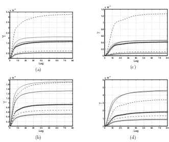
In Fig. 2 a few points stand out. The lag, reported in terms of the grid spac-ing ∆x, at which the asymptotic value is reached is greater for the ∆ = 16η
cases and the approach is uniformly more gradual, indicating greater smooth-ness of the field. This, however, does not mean that the range of subfilter variance values is narrower. On the contrary, the variances of the subfilter variance values are several times greater for the ∆ = 16ηdata at all times an-alyzed. Betweent= 0.1τ andt= 0.3τ (not shown), the variance increases for all calculation methods,. This reflects the transition of the scalar fields from their initial state to one mixed on intermediate scales. By t= 0.7τ the vari-ance of Z′2
calculated from the second order central scheme increases, while it decreases for all other subfilter variance fields. The increase in Var[Z′2
] is much greater for the case evolved using Eq. 1.
In the analysis of Markov fields, coding methods have been used to gen-erate independent data. Essentially, the field is divided into disjoint sets of points containing no neighbors on the grid [2]. Although coding methods are obviously not strictly applicable here, they suggest winnowing the data to eliminate highly correlated pairs of points. In the current case, requiring zero correlation between points thins the data too severely. Instead, values are sampled at intervals of 16∆x apart so that only weak levels of correlation remain. The resulting data is approximated as independent.
0 10 20 30 40 50 60 70 80
Fig. 2. Semivariograms of the subfilter variance field computed with exact DNS variance (black) and modeled variance from filtered DNS scalar (gray) and LES scalars evolved using spectral (gray dots), CD-2 (dashed), CD-4 (black dots), and P-6 (dash-dot) schemes att= 0.7τ. (a) ∆=8η, Eq. 1 (b) ∆=8η, Eq. 2 (c) ∆=16η, Eq. 1 (d) ∆=16η, Eq. 2
3.2 Evolution of subfilter variance distributions
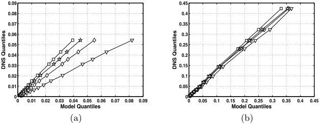
Quantile-quantile (q-q) plots provide a means of comparing two distributions without assuming a parametric form while avoiding ad hoc bin assignments necessary for constructing histograms. Thepquantileζpindicates the value of
a random variableζat which its cumulative distribution function,F, equalsp, i.e. it satisfiesF(ζp) =p. In Fig. 3, quantiles of the modeled subfilter variances
distributions can be largely explained by changes in the scale parameter, which accords with the results of Section 3.1.
In Figs. 3 and 4, symbols indicate the position of specific quantile esti-mates. These are the 0.05, 0.1, 0.2, 0.3, 0.4, 0.5, 0.6, 0.7, 0.8, 0.9, 0.925, 0.95, and 0.975 quantiles. The distribution of subfilter variance values is strongly left-skewed. Results are shown for ∆ = 8η simulations only, as the ∆ = 16η
results are qualitatively very similar.
Initially, the differences between the modeledZ′2quantiles are small for all
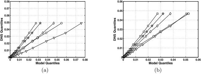
but the highest quantiles examined and agree fairly well with the distribution of exact subfilter variance from the DNS. As the scalar fields evolve, the disparities between the distributions of modeled subfilter variance increase (Fig. 3).
Before pursuing the causes and implications of these findings, it should be recalled that the plots show estimated quantiles, based on a limited sample. Confidence intervals for the data can be obtained through bootstrap tech-niques [4, 3] if we continue to treat the data as independent. Fig. 4 plots differences of the estimated pquantilesZ′2model
p −Z′
2exact
p and their 95
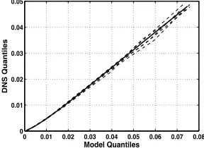
per-cent confidence intervals. These confidence intervals are obtained by forming 1000 random resamples of the original data and repeating the quantile dif-ference calculations for each sample. The results are then sorted in ascending order, with the 25th and 975th values forming the lower and upper bounds. The behavior of the quantile differences is consistent with the hypothesis of a scale change between the modeled and exact differences, with some more complex changes perhaps occurring in the extreme right tails. The confidence intervals of the differences overlap at their edges in several areas, but do sup-port the claim that the second order scheme results in a different subfilter variance distribution than the fourth or sixth order schemes. Fig. 5 provides another indication of the uncertainty of the quantile estimates. In addition to the data used in Fig. 3(a), alternative samples of the CD-2 and exact subfil-ter variance fields, formed by selecting points at the same insubfil-terval but with a different starting point, are plotted as dashed lines. Intersample variabil-ity is clearly evident, but does not meaningfully alter our assessment of the scheme’s performance. Also shown is the result when all points in the field are used for the quantile calculations. As expected, it does not differ greatly from the other estimates for this kind of statistic with this kind of data.
Ina priori tests, lower order schemes produce larger coefficient values by underestimating the gradient-based termMof the closure. In thea posteriori case, evolution using lower order schemes shifts the bulk of the distribution of the Leonard termLto higher values, as shown in Fig. 7(a). A higher value implies greater filtered scalar energy near the cutoff lengthscale, a feature that can be readily inferred from the scalar spectrum (Fig. 1). This result is a direct consequence of the increased errors in finite difference schemes at high wavenumbers, as quantified by the modified wavenumber of the discretization. Although higher values ofL are associated with higher (exact) values ofM, finite difference errors cause underestimation ofMthat roughly balances the error of the scalar evolution (Fig. 7(b)).
0 0.01 0.02 0.03 0.04 0.05 0.06 0.07 0.08 0
0.01 0.02 0.03 0.04 0.05 0.06 0.07 0.08
Model Quantiles
DNS Quantiles
(a)
0 0.01 0.02 0.03 0.04 0.05 0.06
0 0.01 0.02 0.03 0.04 0.05 0.06
Model Quantiles
DNS Quantiles
(b)
Fig. 3. Quantiles of modeled subfilter variance from ∆=8η filtered DNS (circle) and LES using spectral (square), CD-2 (triangle), CD-4 (diamond), and P-6 (star) schemes plotted against quantiles of exact DNS variance at t=0.7τ. (a) Filtered scalar evolved with Eq. 1 (b) Filtered scalar evolved with Eq. 2
4 Conclusions
0 0.1 0.2 0.3 0.4 0.5
−0.01
−0.008
−0.006
−0.004
−0.002 0
Probability
Quantile differences
(a)
0.5 0.6 0.7 0.8 0.9 1
−0.05
−0.04
−0.03
−0.02
−0.01 0 0.01
Probability
Quantile differences
(b)
Fig. 4. Estimated quantile differences (solid lines) and 95% bootstrap confidence intervals (dashed lines) for subfilter variance of ∆=16η, Eq. 2 case att=0.7τ. Exact DNS quantiles are subtracted from quantiles of modeled variance from filtered DNS (circle) and LES using spectral (square), CD-2 (triangle), CD-4 (diamond), and P-6 (star) methods. (a) 0.05 to 0.5 quantiles (b) 0.5 to 0.975 quantiles
0 0.01 0.02 0.03 0.04 0.05 0.06 0.07 0.08 0
0.01 0.02 0.03 0.04 0.05
Model Quantiles
DNS Quantiles
Fig. 5. Quantile plots of data from CD-2 and exact subfilter variance fields of equivalent size and spacing to the samples used in Fig. 3(a) (dashed) as well as to plot formed from full data set (solid)
Model comparisons were made on the basis of estimated one-point statis-tics. Values of subfilter variance were found to be highly correlated over a distance of several grid points, which can be problematic when using statisti-cal methods that assume independent data. Although the statististatisti-cal estimates considered here did not appear to be affected by the correlation of the data, this issue seems to warrant further attention for other quantities of interest in subfilter model tests. A method for estimating confidence intervals of the sam-ple statistics was presented, which can guide expectations when generalizing the results of tests to other data.
References
0.1 0.2 0.3 0.4 0.5 0.6 0.7 0.8 0.9
Fig. 6.Model coefficientCplotted against normalized timeτ. Results are for filtered DNS (circle) and LES using spectral (square), CD-2 (triangle), CD-4 (diamond), and P-6 (star) methods to solve Eq. 1 (open symbols) and Eq. 2 (filled symbols). (a) ∆=8η(b) ∆=16η
Fig. 7.Quantiles of terms of the dynamic closure att=0.7τ for ∆=8ηfiltered scalars evolved with Eq. 2 using spectral (square), CD-2 (triangle), CD-4 (diamond), and P-6 (star) schemes are plotted against quantiles of terms evaluated from filtered DNS. (a)L(b)M
2. Besag J (1974) J Roy Stat Soc B Met 36:192-236
3. Cressie NAC (1993) Statistics for Spatial Data. Wiley, New York 4. Ferro CAT, Hannachi A, Stephenson DB (2005) J Climate 18:4344–4354 5. Kaul CM, Raman V, Balarac G, Pitsch H (2009) Phys Fluids 21:055102 6. Kaul CM, Raman V, Balarac G, Pitsch H (2009) Numerical errors in scalar
variance models for large eddy simulation, Sixth International Symposium on Turbulence and Shear Flow Phenomena, Seoul, Korea
7. Kravchenko AG, Moin P (1997) J Comput Phys 131:310-322
8. Moin P, Squires K, Cabot W, Lee S (1991) Phys Fluids A 3:2746-2757 9. Pierce CD, Moin P (1998) Phys Fluids 10:3041-3044