AIRBORNE HYPERSPECTRAL REMOTE SENSING FOR IDENTIFICATION
GRASSLAND VEGETATION
P. Burai a *, T. Tomor a, Bekő L.a, B. Deák b
a Research Institute of Remote Sensing and Rural Development, Karoly Robert College, Gyöngyös, Hungary – (pburai, tomor, lbeko)@karolyrobert.com
b MTA-DE Biodiversity and Ecosystem Services Research Group, Debrecen, Hungary – [email protected]
WG VII/3
KEY WORDS: Vegetation Mapping, Hyperspectral, Image Classification, Maximum Likelihood Classifier, Random Forest, Support Vector Machine, Open Landscape
ABSTRACT:
In our study we classified grassland vegetation types of an alkali landscape (Eastern Hungary), using different image classification methods for hyperspectral data. Our aim was to test the applicability of hyperspectral data in this complex system using various image classification methods. To reach the highest classification accuracy, we compared the performance of traditional image classifiers, machine learning algorithm, feature extraction (MNF-transformation) and various sizes of training dataset. Hyperspectral images were acquired by an AISA EAGLE II hyperspectral sensor of 128 contiguous bands (400–1000 nm), a spectral sampling of 5 nm bandwidth and a ground pixel size of 1 m. We used twenty vegetation classes which were compiled based on the characteristic dominant species, canopy height, and total vegetation cover. Image classification was applied to the original and MNF (minimum noise fraction) transformed dataset using various training sample sizes between 10 and 30 pixels. In the case of the original bands, both SVM and RF classifiers provided high accuracy for almost all classes irrespectively of the number of the training pixels. We found that SVM and RF produced the best accuracy with the first nine MNF transformed bands. Our results suggest that in complex open landscapes, application of SVM can be a feasible solution, as this method provides higher accuracies compared to RF and MLC. SVM was not sensitive for the size of the training samples, which makes it an adequate tool for cases when the available number of training pixels are limited for some classes.
1. INTRODUCTION
Hyperspectral data is widely applied for monitoring of the environment (Thenkabail, 2011; Adam et al., 2010). Airborne hyperspectral imagery can provide multiple narrow and contiguous spectral bands of less than 10 nm with a high geometric resolution (0.5–1 m). Hyperspectral imagery was proven to be a suitable method for a detailed vegetation classification based on the dominant or subdominant genera or species (Huang and Asner, 2009; Mirik et al., 2013). For processing hyperspectral data it is important to reduce the high dimensionality and inherent multi-collinearity of datasets. Several advanced feature extraction techniques (e.g., MNF, PCA) can be applied for this purpose (Plaza et al., 2009, Green et al., 1988; Landgrebe, 2003).
Alkali habitats of the Pannonian Biogeographical region are one of the most extended semi-natural open landscapes of the European Union. Given their complexity, open alkali landscapes provide an excellent possibility for testing the potential of remote sensing in mapping extended areas with a high spatial complexity (Alexander et al., 2015; Zlinszky et al., 2015). Alkali landscapes are characterized by a fine-scale mosaic of different vegetation types. The most typical ones are open alkali grassland vegetation, dry alkali grasslands, tall-grass meadows, and sedge vegetation together with alkali and non-alkali marshes (Deák et al., 2014a, 2015; Kelemen et al., 2013, 2015). Alkali landscapes are characterised by a fine-scale mosaic of various vegetation types with similar characteristics
(biomass, vegetation structure and environmental conditions; Deák et al., 2014b, Valkó et al., 2014), thus their classification using remote sensing data is often challenging. Our aim was to test the applicability of hyperspectral data in this complex system using various image classification methods. To reach the highest classification accuracy, we compared the performance of traditional image classifiers, machine learning algorithm, feature extraction (MNF-transformation) and various sizes of training dataset.
2. METHODOLOGY
2.1 Study area
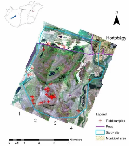
Our study area is located in Pentezug-puszta (N 47°34' E 21° 6'). Pentezug - which is an integral part of the Hortobágy National Park (East-Hungary) – has the area of 23.49 hectares (Figure 1). It harbours a diverse landscape, which represents most of the typical alkali vegetation types: alkali steppes, open alkali grasslands, alkali meadows and marshes. In our study we excluded the roads, buildings, and woody vegetation.
2.2 Airborne and Field Data Collection
For collecting hyperspectral data we used an Aisa EAGLE II type hyperspectral sensor with OxTS RT 3003 GPS/INS system. The sensor provided images with 128 contiguous bands (400-1000 nm), a spectral sampling of 5 nm bandwidth, and a ground pixel size of 1 m. The flight took place in good weather conditions from 09:11 to 09:53 GMT, on 7th July 2013.
Figure 1. Overview map of the study site. We indicated the positions of field measurement plots in the RGB mosaic of the
hyperspectral image with red cross marks
Reference data was collected from all characteristic and representative vegetation types of the study site in a one-week interval after the flight. Given the fact that in alkali landscapes both the total area, distribution and patch size of different vegetation types generally show a high variability, before the field campaign, we carried out a preliminary survey. During the field survey we enlisted the typical vegetation types and estimated their average patch size and proportion in the study area. During the field survey we surveyed 98 homogenous vegetation patches using a differential GPS. For the calculations based on their relative cover we categorised the species as dominant (>50%) and subdominant (10-50%).
2.3 Vegetation Classes
Our aim was to classify the herbaceous vegetation (grasslands and wetlands) as these vegetation types are the best represented (~ 99.5% of the total area) in our study site. Furthermore these vegetation types have the highest importance for nature conservation and site managers in our study region. We built up twenty vegetation classes (Table 1) for which we used the dominant species, the canopy height and the total vegetation cover of different vegetation types. When it was necessary we used the subdominant species as well for creating distinct classes.
Abbreviation Plant association
CYN Cynodonti-Poëtum angustifoliae
FAC Achilleo-Festucetum pseudovinae
FAR Artemisio-Festucetum pseudovinae
CAM Camphorosmetum annuae
PHO Pholiuro-Plantaginetum
ART secondary alkali open grasslands
ELY Agrostio-Alopecuretum with Elymus
ALO Agrostio-Alopecuretum
BEC Agrostio-Beckmannietum
ACI weedy Agrostio-Alopecuretum
CAR Carex spp.
GLY Glycerietum maximae
TYP Typhaetum angustifoliae
SAL Salvinio-Spirodeletum
BOL Bolboschoenetum maritimae
SCH Schoenoplectum tabernaemontani
PHR Phragmitetum communis
FMM mown Agrostio-Alopecuretum
ARA* fallow
MUD muddy surface
Table 1. Abbreviations of vegetation classes and the name of the studied plant association
For testing the effect of pixel numbers on image classification we selected reduced training datasets of 10, 15, 20, 25 and 30 pixels from each vegetation class. We used four categories -corresponding to the available number of field samples (pixels) - for calculating validation datasets (Burai et al. 2015). We aimed to have a ratio of 50-50% of field samples and validation dataset. Pixels were selected randomly from the field samples. The same validation dataset was used for all analyses.
2.4 Image Classification
ENVI/IDL 5.0 (Exelis, Inc., Boulder, CO, USA) and EnMap Box (Rabe et al., 2013) softwares were used to classify hyperspectral images. We tested the efficiency of three supervised classification methods (MLC, RF and SVM) which are frequently used for vegetation mapping (Mirik et al. 2013, Huang & Asner, 2009, Lawrence et al., 2006).
3. RESULTS
3.1 Image Classification Using Original Spectral Bands
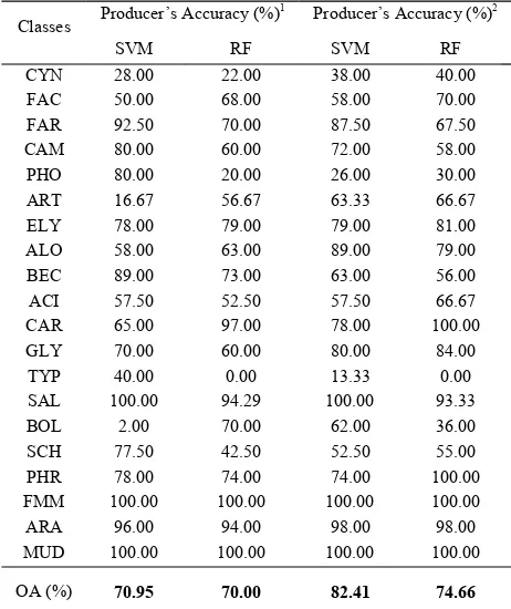
We used SVM and RF with the original dataset for supervised classification. We did not apply MLC on original bands, as it would need at least n+1 training data per class. Image classification was repeated five times with random sampling methods. Given the limited availability of training pixels (from the classes poorly represented in the field) the maximum size of randomly selected training pixels was 30. The overall accuracies provided by SVM and RF classifiers increased slightly with increasing number of training pixels (Table 2 and Figure 2). We found that the standard errors of overall accuracies were similarly low irrespectively from the number of training pixels.
Classes Producer’s Accuracy (%)
1 Producer’s Accuracy (%)2
SVM RF SVM RF
CYN 28.00 22.00 38.00 40.00
FAC 50.00 68.00 58.00 70.00
FAR 92.50 70.00 87.50 67.50
CAM 80.00 60.00 72.00 58.00
PHO 80.00 20.00 26.00 30.00
ART 16.67 56.67 63.33 66.67
ELY 78.00 79.00 79.00 81.00
ALO 58.00 63.00 89.00 79.00
BEC 89.00 73.00 63.00 56.00
ACI 57.50 52.50 57.50 66.67
CAR 65.00 97.00 78.00 100.00
GLY 70.00 60.00 80.00 84.00
TYP 40.00 0.00 13.33 0.00
SAL 100.00 94.29 100.00 93.33
BOL 2.00 70.00 62.00 36.00
SCH 77.50 42.50 52.50 55.00
PHR 78.00 74.00 74.00 100.00
FMM 100.00 100.00 100.00 100.00
ARA 96.00 94.00 98.00 98.00
MUD 100.00 100.00 100.00 100.00
OA (%) 70.95 70.00 82.41 74.66
Table 2. Classification accuracies in respect to the SVM and RF classifiers using original bands (128) and random training
samples, (1) 10 and (2) 30 pixels.
Both classifiers provided their best performance using original bands with 30 training pixels (SVM: 72.84%; RF: 72.89%). SVM classifier using 30 training pixels provided high accuracies for several classes: CYN, FAR, ELY, ALO, BEC, CAR, GLY, SAL, FMM, ARA and MUD (Figure 2).
Figure 2. Overall accuracies of RF and the SVM classifiers. Original bands and different number of random training pixels (N = 10; 15; 20; 25 or 30) were used from each vegetation class
(mean ± SD).
3.2 Image Classification Using MNF-Transformed Bands
Application of the MNF 1–9 transformed bands provided the highest overall accuracies for both SVM and RF classifiers (SVM: 82.06%; RF: 79.14%); additional features over the first 9 MNF bands did not significantly improve the accuracy. We found that when using MLC additional features over the 1-5 MNF bands could not improve the accuracy. Even though each classifier provided considerably high overall accuracies with 30 random training pixels (SVM: 82.06%; RF: 79.14%; MLC: 80.78%) (Figure 3 and Figure 4), we found that only the SVM and RF classifiers had a good performance even with a low number of training pixels. SVM provided an overall accuracy of 79.57% and RF provided 76.55% when using 10 random training pixels, while the accuracy of the MLC classifier decreased considerably (Table 3). MLC classifier using less than 20 training pixels provided low classification accuracies (with high standard error).
Figure 3. Overall accuracies of SVM, RF and MLC classifiers using nine MNF-transformed bands and different number of random training pixels (N = 10; 15; 20; 25 or 30) from each
Figure 4. Vegetation map (A) of the study site produced using SVM classification with 30 random training pixels per class.
Classes
Producer’s Accuracy (%)1 Producer’s Accuracy (%)2
SVM RF MLC SVM RF MLC
CYN 84.00 48.00 26.00 82.00 52.00 22.00
FAC 50.00 52.00 50.00 56.00 70.00 70.00
FAR 95.00 70.00 42.50 90.00 37.50 52.50
CAM 54.00 56.00 62.00 54.00 52.00 48.00
PHO 26.00 30.00 42.00 24.00 10.00 36.00
ART 63.33 93.33 80.00 56.67 83.33 60.00
ELY 95.00 91.00 93.00 94.00 92.00 3.00
ALO 99.00 96.00 100.00 95.00 93.00 86.00
BEC 99.00 91.00 87.00 99.00 100.00 94.00
ACI 57.50 62.50 80.00 57.50 65.00 30.00
CAR 97.00 94.00 100.00 89.00 97.00 81.00
GLY 100.00 98.00 98.00 90.00 94.00 30.00
TYP 8.00 4.00 28.00 24.00 16.00 0.00
SAL 100.00 100.00 100.00 100.00 100.00 0.00
BOL 42.00 46.00 66.00 44.00 40.00 26.00
SCH 72.50 80.00 87.50 47.50 42.50 60.00
PHR 68.00 64.00 80.00 70.00 58.00 44.00
FMM 100.00 100.00 100.00 100.00 100.00 85.00 ARA 100.00 100.00 90.00 100.00 92.00 100.00 MUD 100.00 100.00 100.00 100.00 100.00 0.00
OA
(%) 82.06 79.14 80.78 79.57 76.55 52.56 Table 3. Producer’s accuracy (%) of the classes using SVM, MLC and RF classifiers with 9 MNF-transformed bands and 30 (1) and 10 (2) random training pixels.
We found that ELY, ALO, BEC, CAR, GLY, SAL, FMM, ARA and MUD classes were classified with a high accuracy by all classifiers, when using 30 random training pixels. We found that the tested classifiers provided considerably different accuracies for the CYN, FAR, ACI and TYP classes.
4. DISCUSSION training pixels. In this case the SVM had a considerably higher overall performance (82.41%) compared to the RF (74.66%). However classification with original bands resulted in a high Producer's accuracy for most classes, in certain cases (PHO, TYP and BOL) we detected low accuracies. In these cases most of the pixels were assigned to another class with similar attributes (ratio of open soil surface or the amount of biomass). In order to select the optimal number of transformed features, we used SVM classification on 2-15 MNF-transformed bands. We found that the SVM algorithm with the first nine MNF-transformed bands produced the best accuracy. Further features did not increase the classification accuracy considerably. Classification accuracies of SVM and RF were considerably higher compared to the MLC classification when using smaller training datasets due to the instability of the estimated covariance matrix of MLC. Based on our results, in complex landscapes application of SVM can be a feasible solution, as it provided the highest accuracies compared to the RF and MLC. SVM was not sensitive for the size of the training samples, which makes it an adequate tool for cases when the available number of training pixels are limited for some classes.
ACKNOWLEDGEMENTS
This research was conducted in the project entitled “TÁMOP-4.2.2.D-15/1/ KONV-2015-0010”
REFERENCES
Adam, E., Mutanga, O., Rugege, D. 2010. Multispectral and hyperspectral remote sensing for identification and mapping of wetland vegetation: A review. Wetlands Ecology Management,
18 (3), pp. 281−296.
Alexander, C., Deák, B., Kania, A., Mücke, W., Heilmeier, H. 2015. Classification of vegetation in an open landscape using full-waveform airborne laser scanner data. International Journal of Applied Earth Observations and Geoinformation,
DOI: 10.1016/j.jag.2015.04.014
Burai, P., Deák, B., Valkó, O., Tomor, T. 2015. Classification of herbaceous vegetation using airborne hyperspectral imagery remote. Remote Sensing, 7 (2), pp. 2046–2066.
Green, A.A., Berman, M., Switzer, P., Craig, M.D., 1988. A transformation for ordering multispectral data in terms of image quality with implications for noise removal, IEEE Transactions
on Geoscience and Remote Sensing, 26 (1), pp. 65–74.
Huang, C. and Asner, G.P., 2009. Applications of remote sensing to alien invasive plant studies. Sensors, 9 (6), pp. 4869– 4889.
Kelemen, A., Török, P., Valkó, O., Deák, B., Tóth, K., Tóthmérész, B., 2015: Both facilitation and limiting similarity shape the species coexistence in dry alkali grasslands.
Ecological Complexity, 21 (1), pp. 34–38.
Kelemen, A., Török, P., Valkó, O., Miglécz, T., Tóthmérész, B., 2013: Mechanisms shaping plant biomass and species richness: plant strategies and litter effect in alkali and loess grasslands. Journal of Vegetation Science, 24 (6), pp. 1195– 1203.
Landgrebe, D.A. 2003. Signal Theory Methods in Multispectral Remote Sensing; John Wiley & Sons: New York, NY, USA, p. 503.
Lawrence, R., Wood, S., Sheley, R. 2006. Mapping invasive plants using hyperspectral imagery and Breiman Cutler classifications (RandomForest). Remote Sensing of
Environment,100 (3), pp. 356–362.
Mirik, M., Ansley, R.J., Steddom, K., Jones, D.C., Rush, C.M., Michels, G.J., and Elliott, N.C. 2013. Remote distinction of a noxious weed (musk thistle: Carduus nutans) using airborne hyperspectral imagery and the Support Vector Machine Classifier. Remote Sensing, 5 (2), pp. 612–630.
Plaza, A., Benediktsson, J.A., Boardman, J.W., Brazile, J., Bruzzone, L., Camps-Valls, G., Chanussot, J., Fauvel, M., Gamba, P., Gualtieri, A., Marconcini M., Tilton, J.C., Trianni G. 2009. Recent advances in techniques for hyperspectral image processing. Remote Sensing of Environment, 113 (1), pp. 110– 122.
Rabe, A., Jakimow, B., Held, M., van der Linden, S. and Hostert, P. 2014. EnMAP-Box, Version 2.0. http://www.enmap.org (28 Jan. 2015).
Thenkabail, P.S., 2011. Hyperspectral Remote Sensing of Vegetation; Taylor and Francis: New York, NY, USA, p. 781.
Valkó, O., Tóthmérész, B., Kelemen, A., Simon, E., Miglécz, T., Lukács, B., Török, P., 2014. Environmental factors driving vegetation and seed bank diversity in alkali grasslands.
Agriculture, Ecosystems & Environment, 182, pp. 80–87.
Zlinszky, A., Deák, B., Kania, A., Schroiff, A., Pfeifer, N. 2015. Mapping Natura 2000 Habitat Conservation Status in a Pannonic Salt Steppe with Airborne Laser Scanning. Remote