www.elsevier.comrlocateratmos
On the influence of surface heterogeneity on latent
heat fluxes and stratus properties
Katja Friedrich
1, Nicole Molders
¨
)LIM-Institut fur Meteorologie, Uni¨ Õersitat Leipzig, Stephanstraße 3, D-04103 Leipzig, Germany¨ Received 26 August 1999; received in revised form 16 November 1999; accepted 6 December 1999
Abstract
A mesoscale atmospheric model is used to examine the three-dimensional structure and evolution of low extended stratus over various synthetic landscapes of different heterogeneity in mid-latitudes in spring. The simulation results substantiate that surface heterogeneity nonlinearly influences the distributions of latent heat fluxes, vertical motions, and cloud-water presupposed the length of the patches of equal surface type is about 10 km or larger than that. For low degrees
Ž .
of heterogeneity large patch sizes , a great coverage by lowly evapotranspiring, but strongly heating patches may enhance vertical motion. Moreover, this constellation may increase the cloud-water amount of low extended stratus as compared to that of the other heterogeneous landscapes or that with the highest domain-averaged daily sum of latent heat fluxes. Although there exists a relationship between the degree of heterogeneity and the modulation of latent heat fluxes as well as cloud-water amount, the kind of surface characteristics is also important for the modulation of the properties of low extended stratus.q2000 Elsevier Science B.V. All rights
reserved.
Keywords: Degree of heterogeneity; Latent heat fluxes; Low extended stratus; Mesoscale modeling; Surface
atmosphere interaction
1. Introduction
Flying over a landscape in mid-latitudes presents a fantastic view of patchy fields with various surface properties and different sizes. Obviously, this surface heterogeneity
)Corresponding author. Tel.:q49-341-9732-872; fax:q49-341-9732-899.
Ž .
E-mail address: [email protected] N. Molders .¨
1
Present affiliation: DLR, Institut fur Physik der Atmosphare, Oberpfaffenhofen, Postfach 1116, 82230¨ ¨
Wessling, Germany.
0169-8095r00r$ - see front matterq2000 Elsevier Science B.V. All rights reserved. Ž .
can be significant at the mesoscale or global scale. The varying nature and structure of land-surface result in different fluxes of momentum, water vapor, matter, and heat due to differences in water availability, surface temperature, plant and soil characteristics as
Ž .
well as hill slopes e.g., Li and Avissar, 1994 . Thus, the meteorological processes
Ž .
taking place in the atmospheric boundary layer ABL and at the interface earth–atmo-sphere are, among others, governed by surface characteristics and surface discontinu-ities. This impact is exacerbated, for instance, by moistening of the ABL through
Ž .
evapotranspiration, the rising of lighter, moist air as compared with dry air , and the additional ascending motion induced by surface thermal heterogeneity. Therefore, it has to be expected that the degree of heterogeneity may affect the water and energy fluxes as well as cloud formation.
The impact of surface characteristics and discontinuities on the ABL was investigated
Ž
in many theoretical and numerical studies as well as field experiments e.g., Anthes,
1984; Pinty et al., 1989; Mahrt et al., 1994; Zhong and Doran, 1995; Molders and
¨
.
Raabe, 1996 . Investigating interactions between land cover and cloud cover by means
Ž .
of GOES satellite data on a 18=18 grid, O’Neal 1996 hypothesized that it could be
possible to define a measure denoted as ‘‘degree of surface heterogeneity’’ within larger areas to test whether areas with greater land-surface heterogeneity have significantly less or larger cloud cover. The intensity of thermally induced mesoscale circulations between vegetated and bare soil areas — so-called vegetation breezes — was found to be
Ž
directly related to the characteristics of the bare soil and surface fluxes Mahrt et al.,
.
1994; Hong et al., 1995 . In general, upward motion in such mesoscale circulations is
Ž .
stronger than thermal cells induced by turbulence e.g., Seth and Giorgi, 1996 . Their ability to transport moist, warm air upward increases the amount of water that can be condensed and precipitated. In a relatively dry atmosphere, clouds and precipitation
Ž
appear to be randomly distributed when the domain is homogeneous e.g., Avissar and
.
Liu, 1996; Seth and Giorgi, 1996 . However, when the landscape structure triggers the formation of mesoscale circulations, they concentrate on the originally dry parts of the domain. A negative feedback is created, which tends to eliminate the effect of the
Ž
landscape discontinuities and spatially homogenize soil moisture content e.g., Avissar
.
and Liu, 1996 .
Most studies on the atmospheric impact of land-surface heterogeneity were carried
Ž
out for arid or semiarid regions and convective precipitating clouds e.g., Anthes, 1984;
.
Mahrt et al., 1994; Zhong and Doran, 1995 . In these regions, it is of interest, for instance, for water management, irrigation purposes or limitations of grazing, whether there exist land-use pattern distributions that favor cloud formation. Even in high mid-latitudes, where, however, the atmosphere is usually relatively humid, the analyses of aircraft data show that moisture variability is likely to have an impact on relative
Ž .
Ž
in mid-latitudes, land-surface conditions are anthropogenically altered e.g., through urbanization, deforestation and afforestation, subsidy politics, open-pit mining and
.
recultivation of open-pit mines, etc. . These land-use changes go along with modifica-tions of surface heterogeneity. Since low extended stratus may significantly alter
Ž .
photolysis rates Molders et al., 1995 as well as evapotranspiration, and, thus, ground-
¨
Žwater recharge, land-use changes may not only affect the water and energy cycle e.g.,
.
Molders, 1998 , but also the trace gas concentrations. Moreover, since in mid-latitudes,
¨
extended low stratus is often supercooled, here, land-use changes that contribute to enhance stratus should be avoided in areas of airports due to the danger of icing.
2. Model description and initialization
The nonhydrostatic meteorological model GEesthacht’s SImulation Model of the
Ž .
Atmosphere GESIMA, Kapitza and Eppel, 1992; Eppel et al., 1995 is used in our study. Its dynamical part is based on the anelastic equations.
The physical features of the cloud module are based upon a five water-class
Ž .
cloud-parameterization scheme Molders et al., 1997 . In this scheme, saturation adjust-
¨
Ž .
ment follows Lord et al. 1984 . Note that, in the case of low extended stratus, as investigated in our study, condensation and evaporation of cloud-water are the cloud-mi-crophysical processes of most importance.
In the long-wave spectral range, the radiative transfer equation is solved in a simplified two-stream approximation that transforms the radiation flux into an upward
Ž .
and downward one Eppel et al., 1995 . These fluxes are coupled by their values at the upper and lower boundaries. To get reliable upper model boundary fluxes, 10 additional model layers are added at the top of the computational domain of the model. The mean spectral heating is calculated by the divergence of the net long-wave radiation flux
ŽEppel et al., 1995 . The spectral extinction coefficients depend on pressure height and. Ž .
Ž .
temperature. In accord with Buykov and Khvorostyanov 1977 , a wavelength-indepen-dent value is assumed for the extinction coefficients of liquid water. Outside the window region, water vapor and liquid-water absorption are taken into account. The transmission is approximated by a sum of exponential terms adjusted to the results of a statistical
Ž .
band model for more details, see Eppel et al., 1995 . In the short-wave spectral range, only scattering processes are considered, leading to a simple parameterization of the
Ž .
solar flux at the surface see Claussen, 1988; Eppel et al., 1995 . In the case of clouds,
Ž .
the transmission function is formulated in accord with Stephens 1978 . In doing so, the optical thickness of a cloud is considered as a function of liquid-water path by
Ž
integrating the cloud substance densities which are predicted by the
cloud-parameteriza-.
tion scheme from the surface to model top.
Ž .
The treatment of the soilrvegetationratmosphere interaction follows Deardorff 1978
Žsee also Eppel et al., 1995; Molders, 1998 . Herein, homogeneous soil- and land-surface
¨
.characteristics are assumed within a grid cell. A force-restore method determines soil-wetness factors. At the surface, the fluxes of sensible and latent heat are calculated applying a bulk formulation. Transpiration of plants is considered by a Jarvis-type
Ž .
()
K.
Friedrich,
N.
Molders
r
Atmospheric
Research
54
2000
59
–
85
¨
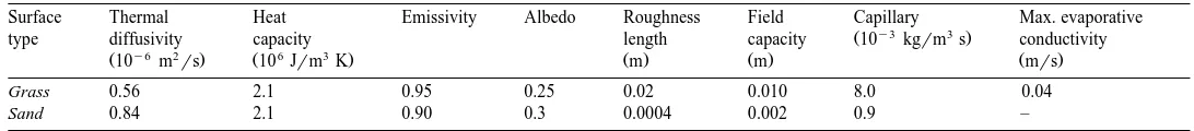
Table 1
Plant- and soil-specific parameters as used in this study
Surface Thermal Heat Emissivity Albedo Roughness Field Capillary Max. evaporative
y3 3
Ž .
type diffusivity capacity length capacity 10 kgrm s conductivity
y6 2 6 3
Ž10 m rs. Ž10 Jrm K. Ž .m Ž .m Žmrs.
Grass 0.56 2.1 0.95 0.25 0.02 0.010 8.0 0.04
Ž .
diffusion equation Claussen, 1988; Eppel et al., 1995 where, at 1-m depth, soil temperature is held constant at the climatological value. The plant- and soil-specific parameters used in this study are listed in Table 1. The surface stress and near-surface fluxes of heat and water vapor are expressed in terms of dimensionless drag-and-transfer
Ž .
coefficients utilizing a parametric model Kramm et al., 1995 .
The turbulent flux of momentum for the region above the surface layer is calculated by a one-and-a-half-order closure scheme. The elements of the eddy-diffusivity tensor are expressed by the vertical eddy diffusivity, KM, V, and horizontal diffusivity, KM,H. The latter is also related to KM, V by the simple linear relationship, KM,Hs2.3 KM,V.
Ž .
KM, V is expressed by the turbulent kinetic energy TKE and mixing length, l, using the
Kolmogorov–Prandtl relation where the mixing length is parameterized by Blackadar’s
Ž1962 approach, slightly modified by Mellor and Yamada 1974 . The turbulent fluxes. Ž .
of sensible heat and water vapor for that region are expressed as functions of KM, V and the turbulent Prandtl number, PrtsKM,VrKH,V, and turbulent Schmidt number, Scts
KM, VrKE,V, respectively. These characteristic numbers depend on the thermal
stratifica-Ž .
tion. They are derived from the local stability functions of Businger et al. 1971 and the assumption that SctsPr . To determine the TKE, an additional budget equation for thatt
Ž
quantity is solved, where the energy production due to horizontal shear is neglected for
.
more detail, see Kapitza and Eppel, 1992 .
The model is initialized using profiles of air temperature and humidity typical for a
Ž .
day with extended low stratus in spring Fig. 1 . Surface pressure is 1031.2 hPa. In the calculation of radiation, a geographical latitude of 51.58N and the 15 May are assumed. Initial soil wetness factor is set equal to 0.5. Soil temperature of 1-m depth is set equal to 280.1 K.
The simulations are integrated for 24 h where the first 6 h serve as the adjusting
Ž . 2
phase. The inner model domain stest domain encompasses 75=75 km with a
horizontal grid resolution of 5=5 km2. The vertical resolution varies from 20 m close
Ž . Ž
Fig. 1. Initial profiles of specific humidity qv in grkg, u- andÕ-component of wind vector in mrs upper
. Ž . Ž .
to the ground to 1 km at the top, which is located in 12-km height. Eight levels are located below the 2-km height and nine are above. Homogeneously flat terrain is assumed for all simulations.
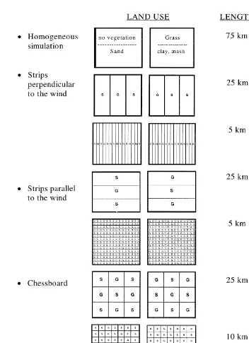
3. Design of the study
Two simulations are performed assuming alternatively a homogeneous cover by sand
Ž .
and grass grown on loamy soil Fig. 2 . These simulations and their results are denoted as HOMS and HOMG, hereafter. Furthermore, sixteen simulations are performed for
Ž .
different patterns of sand and grass Fig. 2 . These simulations and their results are addressed according to the coverage by sand, S, and grass, G, their pattern, and the smallest length of patches given in km. The letters SGS, for instance, stand for a dominance by sand, while GSG stands for a dominance by grass. The patches arranged as stripes parallel or perpendicular to the wind, in form of a checkerboard or a cross are
Ž .
denoted as P, R, C, and X, respectively see Fig. 2 .
In the following discussion, simulation results obtained by assuming the aforemen-tioned landscapes are compared with each other. In doing so, the influence of surface pattern on the water vapor supply to the ABL and on cloud formation as well as the interaction between cloudiness and evapotranspiration are elucidated.
To examine the influence of surface heterogeneity on latent heat fluxes, vertical motion, and the properties of low extended stratus, the degree of surface heterogeneity is
Ž .
defined by Molders, 1999 :
¨
dsFrFmax
Ž .
1for the inner model domain. This measure considers the total length of boundaries,F,
between areas of different surface types in the domain of interest. In the case of a
Ž .
maximum degree of heterogeneity ds1 , each grid cell is also the boundary to another
surface type. The total length of the boundary equalsFma x. In the case of homogeneity,
Ž .
there exists only one surface type and no boundary ds0 . The degree of heterogeneity
as obtained by this measure is listed in Table 2 for the various landscapes.
4. The latent heat fluxes
During the day, the entire domain is totally covered by low-level stratus in all simulations. Since clouds reduce insolation, the turbulent moisture and heat fluxes are weak. At noon, the homogeneously grass-covered domain, for instance, provides a latent
heat flux of 46.4 Wrm2 over the entire domain, while, at the same time, the
homogeneously sand-covered domain provides a latent heat flux of 39.6 Wrm2 over the
Ž .
entire domain Table 2 . The domain-averaged latent heat fluxes of the simulations with
Ž .
heterogeneous surfaces fall between these values Table 2 . Generally, grass-patches provide greater amounts of water vapor to the ABL than sand-patches. Nevertheless, the daily sum of the latent heat fluxes does not correlate to the coverage by grass or the
Ž .
Fig. 2. Schematic view of the land-use distributions applied in the numerical experiments.
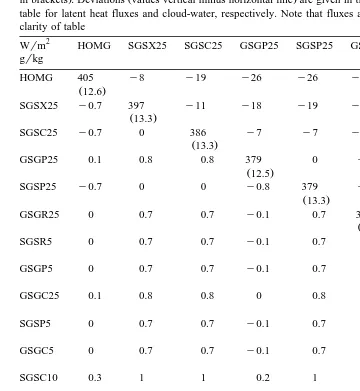
differ-Table 2
Daily sums of domain-averaged latent heat fluxes,ÝL E, domain-averaged latent heat flux at 1300 LT,v ÝL Ev Ž13 , coverage by grass, C, size of the largest grass-covered patch, A, and degree of heterogeneity,. d, for all simulations
2 2 2
Ž . Ž . Ž . Ž . Ž .
Simulation ÝL E Wv rm ÝL E 13v Wrm C % A km d
HOMG 404.6 46.4 100.0 5625 0.00
SGSX25 396.9 41.7 44.4 625 0.16
SGSC25 386.1 43.2 44.4 625 0.20
GSGP25 379.3 43.7 66.7 1875 0.13
SGSP25 378.5 42.8 33.3 1875 0.13
GSGR25 373.6 43.7 66.7 1875 0.13
SGSR5 370.1 43.3 46.7 375 0.53
GSGP5 368.9 43.1 53.3 375 0.53
GSGC25 368.6 42.6 55.6 625 0.20
SGSP5 368.4 43.1 46.7 375 0.53
GSGC5 366.1 42.7 50.2 25 1.00
SGSC10 366.0 42.5 48.0 150 0.47
GSGC10 361.8 42.8 52.0 150 0.47
GSGX25 358.9 44.4 55.6 3125 0.16
SGSC5 353.0 42.2 49.8 25 1.00
SGSR25 345.3 41.8 33.3 1875 0.13
GSGR5 343.9 41.7 53.3 375 0.53
HOMS 316.6 39.6 0.0 0 0.00
ences in water-vapor supply result from the different surface characteristics of grass and
Ž . Ž .
sand Tables 1, 2 and different surface arrangements Fig. 2 . Here, the different albedo, for instance, leads to differences in net radiation. Hence, incoming energy is differently partitioned into the fluxes of sensible and latent heat. Secondary differences result from the modified micrometeorological condition that again affects the heat fluxes. Thus, water supply and moisture transport into the ABL differ too. Therefore, with progressing integration time, further differences may arise from the altered thermal stratification, cloudiness, net radiation reaching the surface and, hence, modified evapo-transpiration, as well as due to differences in the advection of momentum, heat, and moisture. Moreover, at cloud top, the different cloud-water amount leads to changes in
Žlong-wave radiative cooling that again slightly affect the microphysics of the stratus..
Although at the tops of low extended stratus, the impact of surface heterogeneity on radiative cooling may be of some importance, for brevity, this article is limited to the discussion of the influence of surface heterogeneity on latent heat fluxes, vertical motions, and cloud-water amount.
4.1. Distribution pattern of latent heat fluxes
Surface heterogeneity influences the near-surface atmosphere and flow by the altered
Ž
surface characteristics e.g., albedo, roughness length, emissivity, evaporative
conductiv-.
Že.g., near-surface wind, near-surface temperature and humidity, etc. are modified by.
fluxes when ever a parcel passes a change in the underlying surface. Thus, after passing several alternating patches of grass and sand, the micrometeorological condition over a grass-patch located in the western part of the domain, for instance, slightly differ from those over grass in the eastern part of the domain because of the frequent modulation of the air mass when ever passing a discontinuity. These differences grow with time and with increasing distance from the first change in the underlying surface. The altered micrometeorological properties again modify the sensible and latent heat fluxes. The magnitude to which a surface may coin the air mass depends on the time it rests above the patch and, hence, on the patch size. Thus, if the patch size falls below 10=10 km2
like for SGSR5, GSGR5, SGSP5, GSGP5, SGSC5, and GSGC5, respectively, the flux distribution shows hardly an organized response to the underlying surface. Therefore, the results of these studies are not discussed explicitly. For patch sizes larger than 10-km side-length, for instance, in GSGC25, each patch evokes a discernible and assignable
Ž .
own response. These findings broadly agree with Shuttleworth’s 1988 theoretical considerations.
4.1.1. SGSX25 and GSGX25
Ž .
Rotation of crops may cause differences in surface distribution like SGSX25 Fig. 3
Ž . Ž
and GSGX25 Fig. 4 , for instance. Juxtaposing the results obtained for 12 LT local
.
time by simulations with same degree of surface heterogeneity, and patch arrangement,
Ž .
but inverted distribution of grass and sand e.g., SGSX25 and GSGX25, Figs. 3, 4
Ž
shows that landscapes with large connected grass-patches in this example the cross, Fig.
. Ž .
4 and small isolated sand-patches here the edges of the inner domain may supply more water vapor to the ABL than those of opposite arrangement of grass and sand. In
Fig. 4. Like Fig. 3, but for GSGX25.
GSGX25 and SGSX25, the surface characteristics of the cross-area govern the distribu-tion and magnitude of heat and moisture exchange. At noon, for instance, the maximum
2 Ž .
latent heat flux of SGSX25 amounts more than 46 Wrm over grass Fig. 3 compared
2 Ž .
with more than 50 Wrm over grass in GSGX25 Fig. 4 .
4.1.2. GSGC25 and GSGX25
Comparing the results of simulations with different patch sizes and degree of heterogeneity, but same fractional coverage of grass shows that large connected
grass-Ž
patches may provide higher latent heat fluxes than isolated grass-patches e.g., compare
.
GSGX25 and GSGC25, Figs. 4, 5 . The latent heat fluxes of the grass-patch located in
Ž . 2
the center in GSGC25 Fig. 5 , for instance, amounts less than 46 Wrm , while, in
GSGX25, here, locally more than 50 Wm2 are achieved. Thus, one may conclude that
the mean water vapor supply to the ABL by one patch, among others, depends on its size. These findings mean that the surface characteristic of the largest connected part, in the case of GSGX25, the grass-cross, does not only dominate the latent heat-flux distribution, but also affects the fluxes of the downwind neighbored patches.
Note that in the checkerboard arrangement of GSGC25, the grass-patches provide
Ž .
similar fluxes than those in SGSX25 compare Figs. 3, 5 .
4.1.3. GSGC25 and SGSC10
GSGC25 and SGSC10 are landscapes of different degrees of surface heterogeneity,
Ž .
and different coverage by grass, but similar patch pattern Table 2, Fig. 2 . At noon, for
instance, the latent heat fluxes of GSGC25 and SGSC10 range from 32 Wrm2 to 48
2 Ž .
Wrm in both simulations e.g., Fig. 5 . Like in GSGC25, in SGSC10, the latent heat
Ž .
Fig. 5. Like Fig. 3, but for GSGC25.
4.2. Daily domain aÕerages
The largest differentials in the daily sums of the domain-averaged latent heat fluxes
Ž88 Wrm2. occur between the results of HOMG and HOMS Table 3 . The domain-Ž .
averaged latent heat fluxes of all simulations assuming heterogeneous surfaces range
Ž .
between these two values see also Table 2 . The greatest differential between
simula-tions with heterogeneous surface-cover amounts 53 Wrm2 for SGSX25 and GSGR5.
On the contrary, the daily sums of domain-averaged latent heat fluxes hardly differ for the following pairs: GSGP5 and GSGC25, GSGP25 and SGSP25, as well as GSGC5
Ž .
and SGSC10 Table 3 . The daily sums of the domain-averaged latent heat fluxes do not always grow with increasing coverage by grass, size of the grass-covered patches or
Ž .
degree of heterogeneity Tables 2, 3 .
Ž
The greatest deviations arise between HOMS and nearly all other simulations Table
.
3 . In this homogeneously dry and warm, sandy domain, the incoming energy is partitioned toward higher sensible and lower latent heat fluxes than in the partly grass-covered domains or than in the totally grass-covered domain. Even for small fractional coverage by grass, the latent heat flux increases rapidly as compared to
Ž .
HOMS Table 3 . Out of all the simulations assuming heterogeneous landscapes,
SGSX25 provides the greatest daily sums of the domain-averaged latent heat fluxes
Ž396.9 Wrm , although it has not the largest amount of grass Table 2 . This behavior2. Ž .
may be explained by the oasis effect. The slightly warmer air, due to the stronger heating of sand than of grass, enhances evapotranspiration. In contrast to SGSX25, the daily sum of domain-averaged latent heat fluxes is smaller for the ‘‘inverse landscape’’
Ž .
Table 3
Ž . Ž
Daily sums of the domain-averaged latent heat flux upper values and cloud-water mixing ratio lower values
. Ž .
in brackets . Deviations values vertical minus horizontal line are given in the upper and lower triangle of the table for latent heat fluxes and cloud-water, respectively. Note that fluxes and mixing ratios are rounded for clarity of table
2
Wrm HOMG SGSX25 SGSC25 GSGP25 SGSP25 GSGR25 SGSR5 GSGP5
grkg
HOMG 405 y8 y19 y26 y26 y31 y35 y36
Ž12.6.
SGSX25 y0.7 397 y11 y18 y19 y23 y27 y28
Ž13.3.
Looking at the simulations with checkerboard-like landscapes, in the sand-majorized
Ž .
landscapes with large patch sizes e.g., SGSC25, SGSC10 , the daily sums of domain-averaged latent heat fluxes exceed those of their grass-majorized counter-pairs like in
Ž .
SGSX25 e.g., GSGC25, GSGC10 . Here, SGSC10 and GSGC5 provide the same sum
Ž366 Wrm ; Table 3 . Out of the checkerboard-arranged landscapes, SGSC5 provides2 .
Ž 2 .
GSGC25 SGSP5 GSGC5 SGSC10 GSGC10 GSGX25 SGSC5 SGSR25 GSGR5 HOMS
y36 y37 y39 y39 y43 y46 y52 y60 y61 y88
y28 y29 y31 y31 y35 y38 y44 y52 y53 y80
y17 y18 y20 y20 y24 y27 y33 y41 y42 y69
y10 y11 y13 y13 y17 y20 y26 y34 y35 y62
y10 y11 y13 y13 y17 y20 y26 y34 y35 y62
y5 y6 y8 y8 y12 y15 y21 y29 y30 y57
y1 y2 y4 y4 y8 y11 y17 y25 y26 y53
0 y1 y3 y3 y7 y10 y16 y24 y25 y52
369 y1 y3 y3 y7 y10 y16 y24 y25 y52
Ž12.5.
y0.1 368 y2 y2 y6 y9 y15 y23 y24 y51
Ž12.6.
y0.1 0 366 0 y4 y7 y13 y21 y22 y49
Ž12.6.
0.2 0.3 0.3 366 y4 y7 y13 y21 y22 y49
Ž12.3.
y0.1 0 0 y0.3 362 y3 y9 y17 y18 y45
Ž12.6.
0 0.1 0.1 y0.2 0.1 359 y6 y14 y15 y42
Ž12.5.
y0.2 y0.1 y0.1 y0.4 y0.1 y0.2 353 y8 y9 y36
Ž12.7.
0 0.1 0.1 y0.2 0.1 0 0.2 345 y1.4 y28
Ž12.5.
y0.1 0 0 y0.3 0 y0.1 0.1 y0.1 344 y27
Ž12.6.
0.2 0.3 0.3 0 0.3 0.2 0.4 0.2 0.3 317
Ž12.3.
the sand-dominated checkerboard landscapes, the daily domain-averaged latent heat fluxes are arranged according to the patch size.
Ž
In simulations with stripes orientated parallel to the wind GSGP25, SGSP25,
.
for the same degrees of surface heterogeneity. However, no correlation of the daily sums of domain-averaged latent heat fluxes to patch size and arrangement is found in
Ž .
simulations with stripes perpendicular to the wind GSGR25, SGSR25, GSGR5, SGSR5 . SGSC25 and SGSX25 have the same fractional coverage by grass, but different degree of surface heterogeneity. Thus, in this case, the different sums of
domain-aver-Ž
aged latent heat flux result from the different degrees of surface heterogeneity Tables 2,
.
3 .
All these findings suggest that the orientation of the pattern to the wind and the patch size cause differences in the daily sums of the domain-averaged latent heat fluxes. This
Ž .
broadly agrees with the Molders’ 1999 findings who investigated the sensitivity of the
¨
impact of land-use changes to the direction of wind. Moreover, the results suggest that both the fractional coverage and the degree of heterogeneity concurrently affect the latent heat fluxes.
5. Vertical motions
As discussed before, different surface characteristics and discontinuities may lead to different moistening of low-level atmosphere through transpiration and different air heating. Induced by surface thermal heterogeneity, the ascending motions differ. Note that since the vertical velocities are volume averages representing volumes of the
thickness of the model layer times 5=5 km2, the magnitude of vertical velocity
depends on grid size. Generally, the inclusion of a finer grid increases ability of meteorological models to produce larger vertical motions because small-scale horizontal temperature gradients and velocities can be resolved. To avoid differences resulting from
grid size, in our study, all simulations are performed with the same grid size of 5=5
km2 as pointed out already in Section 2.
In all simulations, vertical velocities do not exceed 0.05 mrs. As mean vertical velocities are small, turbulence, in principle, is an important contributor to vertical transport processes, energetics and physics of low extended stratus. In absolute magni-tude, however, the turbulence level is low in low extended stratus.
The pattern of vertical motions depends on patch distribution, patch size, and modulation of the air mass by upwind surface heterogeneity. Water vapor is transported to higher levels by upward motions. In the ABL, a distinct pattern of ascent and descent only develops for some patch arrangements, namely, SGSX25, GSGC25, SGSC10, and GSGX25. In the following, the vertical motions at 12 LT will be exemplary examined for these simulations.
5.1. SGSX25
In Fig. 6, the vertical wind distribution of SGSX25 is exemplary shown at two
Ž
representative WE cross-sections. In the cross-section at 35 km counted from the
. Ž .
south , sand exists only while, in the cross-section at 60 km counted from the south ,
Ž .
grass dominates Fig. 6 . As pointed out before, sand heats more strongly, but supplies less water vapor to the ABL than grass. Due to the stronger heating upward motions
Ž .
Ž . Ž . Ž .
Fig. 6. WE cross-section at a 60 km and b 35 km both counted from the south of vertical wind distribution in cmrs as simulated by SGSX25. At 60 km, maximum and minimum values are 0.2 andy1.1 cmrs, respectively. At 35 km, maximum value is 0.9 cmrs. The black underlined parts represent grass.
Ž .
and southern grass-dominated part cf. Fig. 6a . Here, however, over sand, the
down-Ž .
ward motions exceed those occurring over grass Fig. 6a .
5.2. GSGX25
Ž .
Despite of the same degree of heterogeneity like SGSX25 Table 2 , in GSGX25, a
Ž .
totally different pattern of vertical motion establishes Figs. 6, 7 . In GSGX25, namely,
Ž . Ž .
ascent occurs in the WE cross-sections at 25 Fig. 7c and 15 km Fig. 7d , while
Ž . Ž
descent is found for the WE cross-sections at 35 Fig. 7b and 60 km Fig. 7a; always
.
counted from the south . In contrast to its inverse counterpart SGSX25, in GSGX25, descent or ascent cannot be related to the surface type dominant in the WE cross-section
Ž . Ž . Ž . Ž . Ž .
Žcf. Fig. 7 . The WE cross-sections at 60 descent and 15 km ascent , for instance, are. Ž . Ž .
both dominated by sand. In the WE cross-sections at 35 km, the descent enhances
Ž .
toward the east Fig. 7 . This different behavior results from the altered heating and evapotranspiring, which modifies thermal stratification and vertical motions. This find-ing means that the surface distribution and patch size, i.e., the degree of heterogeneity, are not the only factor that determines the atmospheric response. Additionally, the kind of surface characteristics plays an important role. The effects of heterogeneity and surface characteristics are juxtaposed in the atmospheric response. The effects may even enhance each other in their impact.
5.3. GSGC25
Ž .
In the case of GSGC25 not shown , the vertical motions are similar to those of SGSX25 for the WE cross-section at 35 and 60 km, because of the same patch
Ž .
distribution here see Fig. 2 . In the area of ascent located between 25 and 50 km
Žcounted from the south , however, ascent is less continuously in GSGC25 than in.
SGSX25 due to the grass-patch in the middle of the domain in GSGC25. Perturbations occur above the borders of different surface types, i.e., the additional grass-patch only slightly modifies the vertical motions.
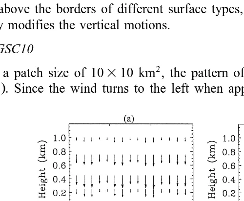
5.4. SGSC10
For a patch size of 10=10 km2, the pattern of vertical motion is quite complicate ŽFig. 8 . Since the wind turns to the left when approaching the surface, it has a more.
Ž . Ž . Ž . Ž . Ž .
northern component than at height. Thus, due to the modulation of the advected air mass by the upwind surface pattern, a different pattern of vertical motions establishes in the
Ž .
northern than in the southern part of the domain e.g., Fig. 8 . In the northern part, for
Ž .
instance, at the WE cross-section at 60 km counted from the south , there is stronger
Ž .
descent over the grass–sand boundary looking from the west . Note that this
cross-sec-Ž .
tion is dominated by grass. At the WE cross-section at 30 km counted from the south
Ž .
ascent is stronger over sand–grass boundary looking from the west . This cross-section is dominated by sand. Based on these findings, one may conclude that descent or ascent depends on the dominant surface type of the cross-section in the northern cross-sections.
Ž .
At the WE cross-section at 10 or 20 km counted from the south , however, the vertical
Ž .
motions cannot be assigned to the dominance of the cross-section e.g., Fig. 8 . Several
Ž .
small areas of descent and ascent establish Fig. 8 . These facts mean that after the air mass has passed alternating relatively small patches several times, a less distinct, but still ‘organized’ behavior of vertical motions establishes.
6. Cloudiness
After reaching the condensation level, water vapor condenses and low extended stratus is formed. In all simulations, the domain is totally covered by extended low stratus during the entire simulation time. The wet adiabatic cooling rates are on the order of 1 Krh. Consequently, radiation and wet adiabatic cooling are approximately equal contributors to low extended stratus.
At noon, cloud bases are at a height of 250 m and cloud tops are at a height of 450 m. In HOMG and HOMS, the cloud-water mixing ratios of the stratus are horizontally uniform throughout the entire simulation. At noon, for instance, the cloud-water of HOMG amounts 0.124 and 0.557 grkg at a height of 250 and 450 m, respectively. At the same time, the cloud-water of HOMS amounts 0.108 and 0.556 grkg at these heights. Obviously, at a height of 450 m, the cloud-water mixing ratios of HOMS and HOMG hardly differ. In the case of heterogeneous surfaces, deviations from these cloud-water values may be related to the effects of heterogeneity on water vapor supply, heating, and vertical motions. Secondary differences result from the modified radiative cooling at cloud top caused by the altered cloud-water distribution. For brevity, these slight effects will not be discussed here.
No apparent response of the low extended stratus to the underlying surface is found for the landscapes with stripes parallel or perpendicular to the wind, no matter of the
Ž .
stripe size SGSR25, GSGR25, SGSP5, GSGP5, SGSR5, GSGR5 . The same is true for
Ž .
landscapes with a patch size of 5 km GSGC5, SGSC5 . Therefore, the results of these simulations are not further discussed.
6.1. Daily sums of domain-aÕeraged cloud-water
When comparing the daily sums of domain-averaged latent heat fluxes with those of
Ž .
cloud-water Table 3 , a correlation is found between the water vapor supply to the atmosphere by turbulent latent heat fluxes and the amount of cloud-water in simulation SGSX25 and SGSC25.
Ž . Ž .
Although simulations SGSX25 44.4% grass , SGSC25 44.4% grass , SGSP25
Ž33.3% grass as well as SGSC5 49.8% grass have less grass than HOMG 100%. Ž . Ž
.
grass , their daily sums of domain-averaged cloud-water are higher due to upward
Ž .
moisture transport enhanced by the stronger surface heating of sand Table 3 . On the
Ž .
other hand, the counterparts of these simulations, namely, GSGC25 55.6% grass ,
Ž . Ž . Ž .
GSGX25 55.6% grass , GSGP25 66.7% grass , and GSGC5 50.2% grass provide
Ž .
lower or equal daily amounts of cloud-water than HOMG Table 2 . This finding means that the combination of heating and evapotranspiring patches may enhance the cloud-water amount of low extended stratus as compared to the case with less surface heating. The differential in the daily sums of domain-averaged cloud-water between GSGC25
Ž .
and SGSC25 as well as between GSGX25 and SGSX25 exceeds 0.8 grkg Table 3 . These differences may suggest that not the amount of land-use, but the land-use distribution, i.e., the degree of surface heterogeneity, plays the major role for cloud-water amount. Comparing the daily sums of domain-averaged cloud-water mixing ratios provided by the simulations with the heterogeneous landscapes, the greatest differences
Ž .
occur for SGSC10 to SGSX25, SGSC25, and SGSP25, respectively Table 3 .
The daily sums of the cloud-water mixing ratios of GSGC10 and SGSC10 broadly
Ž
agree with those of the simulations that assume nearly the same amounts of grass e.g.,
.
GSGC5 50.2%, SGSR5 46.7%, GSGR5 53.3%, GSGP5 53.3%, SGSR5 46.7% . Here, the daily sums of domain-averaged cloud-water differ about 0.3 grkg. The greater importance of the surface distribution than that of the fractional coverage by grass is also manifested by the daily sums of the domain-averaged cloud-water between HOMG and HOMS, which differ 0.3 grkg, although grass supplies more water vapor to the
Ž .
atmosphere than sand e.g., Tables 2, 3 .
6.2. Horizontal distribution of cloud-water
Ž . Ž .
In SGSC10 e.g., Fig. 9a , and SGSX25 e.g., Fig. 9b , the distributions of cloud-water clearly reflect the heterogeneity of the underlying surface in both cloud levels. In
Ž .
GSGC10 not shown , a clear relation of the cloud-water amount to surface heterogene-ity exists for the lower part of the low extended stratus. In the upper part, the relationship is less distinct.
Surprisingly, the structures of the cloud-water distribution provided by GSGC25
Že.g., Fig. 9c are similar to those of SGSX25 e.g., Fig. 9b . The opposite is true for. Ž .
Ž . Ž .
GSGX25 e.g., Fig. 10 and SGSC25 not shown . All other landscapes hardly modulate
Ž
the cloud-water distribution e.g., at 12 LT up to 0.01 grkg at a height of 450 m, and up
.
to 0.005 grkg at a height of 250 m except SGSP25 and GSGP25. In the case of these simulations, a slight, but not distinct modulation parallel to the stripes can be detected
Fig. 9. Distribution of cloud-water mixing-ratio in grkg at 12 LT at a height of 450 m height as simulated by
Ž .a SGSC10, b SGSX25, and c GSGC25, respectively. Grey patches indicate grass and light grey patchesŽ . Ž .
indicate sand, respectively.
with a clear modulation of cloud-water by surface heterogeneity, namely, SGSX25, GSGC25, and SGSC10, respectively. Focus is on the level of maximum cloud-water at 12 LT.
6.2.1. SGSX25
Less cloud-water occurs over both the sand- and grass-patches in SGSX25 than in
Ž .
Fig. 10. Like Fig. 9, but for the distribution of cloud-water mixing-ratio in grkg at 12 LT for GSGX25 at a
Ž . Ž .
height of a 250 m and b 450 m, respectively.
LT. This maximum of cloud-water can be explained as follows: The sand-patches heat
Ž
stronger and provide greater sensible heat fluxes than the grass-patches cf. Friedrich
.
and Molders, 1998 . Thus, air rises over the sand-patches and is replaced by moist air
¨
from the neighbored upwind grass-patches that evapotranspire at a higher rate than sand-patches. Consequently, upward transport is enhanced over the sand-stripe and leads to the increased cloud-water mixing ratios. In SGSX25, less cloud-water is formed
Ž
. Ž
and 25–50 km counted from the south and the southern part in the WE-orientated area
. Ž .
between 0–25 and 25–50 km counted from the south than over grass Fig. 9b . Especially at the northern and southern edges of the domain, there exist higher values above grass-patches than sand-patches.
The effect of the different water vapor supply from grass and sand is visible at a
Ž .
height of 450 m behind the grass–sand boundary Fig. 9b . In the northern part as well as in the southern part, cloud-water decreases behind the grass-patch with 0.005–0.020 grkg and increases after passing the sand with up to 0.010 grkg.
6.2.2. GSGC25
Ž .
In GSGC25, at a height of 450 m, Fig. 9c , the structures in the cloud-water
Ž .
distribution are similar to those of SGSX25 Fig. 9b . Despite of the grass-patch in the center of the domain, in GSGC25, there exists no response to this patch in the distribution of cloud-water. On the contrary, in GSGC25 like in SGSX25, distinct responses in the cloud-water mixing ratio exist at the northern and southern
WE-orien-Ž .
tated stripe 0–25 and 50–75 km counted from the south , providing different values over grass than sand.
6.2.3. SGSC10
Ž .
In SGSC10 Fig. 9a , less cloud-water is formed than in HOMG or HOMS. In the northern most WE-directed stripes, a distinct response to the underlying surface is found with an increase and a decrease of cloud-water after passing either a grass- or a
Ž
sand-patch. In the middle WE-orientated part of the domain between 25 and 50 km
. Ž
counted from the south , maximum cloud-water mixing ratios exceed 0.56 grkg Fig.
.
9a . The clear differences found for the latent heat fluxes over grass and sand are not
Ž .
reflected in the cloud-water distribution Fig. 9a . Seemingly between 20 and 50 km counted from the southern edge of the inner model domain, the cloud-water distribution behaves more like that of a WE-orientated, homogeneously covered surface than that of
Ž .
a heterogeneous surface Fig. 9a . Although, a response is visible, the types of surface do not provide a distinct assignable response in cloud-water mixing ratios.
6.3. Vertical distribution of cloud-water
As aforementioned, on average, the amount of cloud-water increases from cloud-base
Ž . Ž .
to cloud-top e.g., up to 0.4 grkg at noon for all simulations e.g., Fig. 10 . Since there is no relationship between the distributions of the surface and cloud-water for the landscapes with patch lengths of 5 km as well as those with stripes of 25 km width perpendicular to the geostrophic wind direction, the vertical distribution of cloud-water in these landscapes is not further discussed, here.
If the cloud-water distribution clearly shows structures at a height of 250 m, these
Ž
structures will disappear at the 450-m level and new structures will build up e.g., Fig.
.
10 . As pointed out already, in GSGC10, a clear relation between the cloud-water distribution and surface heterogeneity exists only for the lower part of the low extended
Ž .
stratus. In our study, the greatest and most distinct changes of cloud-water distribution
Ž . Ž .
with height are found for GSGX25 e.g., Fig. 10 and GSGC25 not shown at noon, for which these cases are exemplary discussed in detail. For landscapes with large patches
Ž
ascent areas, while at higher levels, maximum values of cloud-water are found e.g., Fig.
.
10 .
6.3.1. GSGX25
In GSGX25, for example, the maximum of cloud-water is found in the middle
Ž .
WE-orientated stripe between 25 and 50 km counted from the south at a height of 250
Ž .
m Fig. 10a . Here, the specific cloud-water values exceed those at the edges by more than 0.020 grkg. Obviously, this middle grass-stripe governs the cloud-water distribu-tion at the southern edges. The lower values of cloud-water occurring over sand-patches
Ž .
at the corners Fig. 10a , may be explained by, on average, lower relative humidity and slightly warmer air occurring over sand than grass. As mentioned before, more water
Ž
evapotranspires over the grass-cross. The steady lifting without disturbance by a change
.
in the underlying surface; Fig. 7 supports the formation of the cloud-water maximum. At a height of 450 m, the cloud-water mixing ratio exceeds 0.560 grkg in the southern
Ž .
part of the domain Fig. 10b . Minimum values of cloud-water mixing ratios amount
Ž .
0.515 grkg at the interface sand–grass at 50 km counted from the south and at the
Ž .
interface grass–sand at 50 km in WE-direction counted from the south; Fig. 10b . Note that the behavior of SGSC25 is similar.
6.3.2. GSGC25
Ž .
Looking at the cloud-water distribution of GSGC25 at 450 m height Fig. 9c , for instance, low cloud-water mixing ratios are found over the northern and southern part where more grass exists than over the middle part and descent occurs. The opposite is
Ž .
true for 250 m not shown . Here, namely, low cloud-water mixing ratios are found over
Ž .
the strong ascent zones at 30–40 km counted from the south at the 250-m level. Greater mixing ratios of cloud-water are found over the decent zones of the
grass-Ž
dominated WE-cross-section between 5–20 and 55–75 km both counted from the
.
south; Fig. 8 left . Note that the behavior of SGSX25 is similar.
6.4. Temporal deÕelopment of cloud-water distribution
In the diurnal course, the amount of cloud-water is related to the magnitude of the sensible and latent heat fluxes with a delay of about 3 h. Increasing latent heat fluxes
Ž .
enhance cloud formation positive feedback . Thus, the liquid-water content of the low extended stratus is maximal at about 15 LT for all simulations. Later on, this enhanced
Ž
cloudiness reduces insolation and, hence, the fluxes of sensible and latent heat negative
.
feedback , which again slightly diminishes cloud-water. At about 18 LT, cloud base starts to sink for most of the simulations.
6.4.1. SGSX25
Ž .
As mentioned already, at 12 LT Fig. 9b , areas of low cloud-water mixing ratios are
Ž .
found in the northern and southern parts above the sand-patches Fig. 9b . The
maximum in the amount of cloud-water occurring over the middle sand-stripe resembles
Ž
a maximum in sensible heat flux at 12 LT above the sand-stripe not shown; for a
.
discussion of the sensible heat fluxes see Friedrich and Molders, 1998 and a maximum
¨
Ž .
in latent heat flux above the grass-corners Fig. 3 . Note that in the northern and
Fig. 11. Like Fig. 9, but for the distribution of cloud-water mixing-ratio in grkg for SGSX25 at a height of
Ž . Ž .
southern sand-patches, the latent heat fluxes increase slightly behind 40 km in
WE-direc-Ž .
tion see Fig. 3 .
Ž
The extension of the area of high cloud-water mixing ratios increases until 15 LT cf.
.
Figs. 9b, 11a . This increase agrees with the maximum of the domain-averaged latent heat flux at 13 LT. The cloud-water maximum that at 12 LT occurs above the
Ž
sand-stripe in WE-direction at the interface grass–sand at 40–60 km counted from the
. Ž .
south , shifts northwards with progressing time cf. Figs. 9b, 11a,b . The same is true for
Ž .
the minimum of cloud-water 0.545–0.540grkg . The distinct upward motion occurring
Ž . Ž .
over sand Fig. 6 breaks down in the late afternoon not shown . Accordingly, the
Ž .
highest values of cloud-water occur at 18 LT in the grass-covered parts Fig. 11b , while over the sandy parts the cloud-water amount decreases rapidly. In the northern and southern parts, the sand-patches do not influence cloud-water amount at the height of 450 m. These findings suggest that surface heterogeneity may not only affect the spatial, but also the temporal development of low extended stratus.
6.4.2. SGSC10
In SGSC10, the cloud-water distribution shows a similar behavior with time than
Ž . Ž .
SGSX25 Figs. 9b, 11 . In SGSC10 Fig. 9a , at a height of 450 m, however, a clear response of cloud-water to surface heterogeneity only exists at 12 LT. The maximum
Ž .
values achieved in the mixing ratios of cloud-water more than 0.560 grkg are found in the WE-orientated area between 25–40 km at 12 LT, 35–55 km at 15 LT, and 40–60
Ž . Ž .
km all counted from the south at 18 LT not shown . Between 15 and 18 LT, the amount of cloud-water decreases agreeing with the decrease of the domain-averaged latent heat flux.
7. Conclusions and outlook
Simulations assuming identical model configurations and meteorological initial condi-tions, but different synthetics landscapes of various degree of heterogeneity are
per-formed with a meso-b-scale meteorological model. Although turbulence and radiative
cooling may play a role for low extended stratus, the main focus is on the impact of surface heterogeneity on latent heat fluxes and the properties of low extended stratus.
Under the meteorological situation assumed in this case study, a clear relationship exists between the underlying surface and the temporal and spatial distribution of cloud-water for a homogeneous patch-size length of 25 km. Herein, the land-use pattern may be squares or crosses, but not stripes that are parallel or perpendicular to the wind.
Patch sizes of 10=10 km2 also provide an obvious response to the underlying surface,
The results substantiate that the amount of cloud-water does not depend primarily on the amount of grass or sand. Large sand-patches are able to force the required upward motions due to great enough fluxes of sensible heat. Nevertheless, adjacent wet patches are necessary to provide sufficient moisture by latent heat fluxes for modification of low extended stratus over the sand-patches, i.e., the moisture transport induced by the surface heterogeneity must be sufficiently great to achieve a modulation of low extended stratus. This means that the fraction of land use, the distribution and the interaction between the neighboring patches concurrently affect cloud-water distribution of a low extended stratus. Consequently, cloud-water mixing ratios may substantially increase if the degree of heterogeneity is low and the fractional coverage of low evapotranspiring, but strongly heating patches slightly exceeds that of the inverse characteristics.
The amount of cloud-water also agrees with the maximum of latent and sensible heat fluxes. Therefore, the amount of cloud-water, independently of the patch size and arrangement, increases in the early afternoon with a temporal offset of 3 h to those of the latent and sensible heat fluxes, and decreases toward the evening hours. The structure of the cloud-water distribution changes depending on the patch arrangement and patch size with increasing simulation time. Thus, it may be concluded that landscape heterogeneity may not only influence the spatial, but also the temporal development of low extended stratus.
A relationship between the maximum of the daily sums of domain-averaged latent
Ž .
heat fluxes and the maximum of the amount of cloud-water Table 2 is only found in SGSX25 and SGSC25. Simulations with well-balanced equal parts of wetrcool and dryrwarm parts with respect to patch size and degree of heterogeneity have increased daily sums of domain-averaged cloud-water as compared to the others. The results of
Ž . Ž .
GSGC25 55.6% grass and GSGX25 55.6% grass , which have the same percentage of grass and sand, but different land-use distribution, suggest that, in some cases, the land-use distribution may be of much more importance than the amount of land use for the daily amount of cloud-water. This fact is also substantiated by the results of simulations wherein the percentage of land use differs only slightly and the daily sums
Ž
of domain-averaged cloud-water differ about 0.3 grkg e.g., GSGC10 and SGSC10 with
.
52% grass and 48% grass, respectively .
Based on all these findings, it may be concluded that surface heterogeneity may influence the properties of low extended stratus via modified fluxes, variables of state, and vertical motions in humid mid-latitudes. Herein, especially, low degree of hetero-geneity in combination with a slight dominance of low evapotranspiring, but strongly heating patches may contribute to higher cloud-water mixing ratios, and, hence, denser stratus. Since stratus is often supercooled, land-use changes leading to landscapes of the aforementioned kind may dramatically increase the risk of icing of airplanes.
Acknowledgements
References
Anthes, R.A., 1984. Enhancement of convectional precipitation by mesoscale variations in vegetative covering in semiarid regions. J. Clim. Appl. Meteorol. 23, 541–554.
Avissar, R., Liu, Y., 1996. Three-dimensional numerical study of shallow convective clouds and precipitation induced by land surface forcing. J. Geophys. Res. 101D, 7499–7518.
Blackadar, A.K., 1962. The vertical distribution of wind and turbulent exchange in a neutral atmosphere. J. Geophys. Res. 67, 3095–3103.
Businger, J.A., Wyngaard, J.C., Izumi, Y., Bradley, E.F., 1971. Flux profile relationship in the atmospheric surface layer. J. Atmos. Sci. 28, 181–189.
Buykov, M.V., Khvorostyanov, V.I., 1977. Formation and evolution of radiation fog and stratus clouds in the
Ž .
atmospheric boundary layer. Izv. Atmos. Oz. Phys. Engl. Ed. 13, 251–260.
Claussen, M., 1988. On the surface energy budget of coastal zones with tidal flats. Contrib. Phys. Atmos. 61, 39–49.
Deardorff, J.W., 1978. Efficient prediction of ground surface temperature and moisture, with inclusion of a layer of vegetation. J. Geophys. Res. 84C, 1889–1903.
Eppel, D.P., Kapitza, H., Claussen, M., Jacob, D., Koch, W., Levkov, L., Mengelkamp, H.-T., Werrmann, N., 1995. The non-hydrostatic mesoscale model GESIMA: Part II. Parameterizations and applications. Contrib. Atmos. Phys. 68, 15–41.
Frech, M., Samuelsson, P., Tjernstrom, M., Jochum, A.M., 1998. Regional surface fluxes over the NOPEX¨
area. J. Hydrol. 212, 155–171.
Friedrich, K., Molders, N., 1998. A numerical case study on the sensitivity of the water- and energy-fluxes to¨
Ž .
the heterogeneity of the distribution of land-use. In: Raabe, A., Arnold, K., Heintzenberg, J. Eds. ,
Ž .
Meteorologische Arbeiten aus Leipzig III , Wiss. Mitt. Leipzig, Vol. 9, pp. 55–74.
Hong, X., Leach, M.J., Raman, S., 1995. Role of vegetation in generation of mesoscale circulation. Atmos. Environ. 29, 2163–2176.
Jarvis, P.G., 1976. The interpretation of the variations in leaf water potential and stomatal conductance found in canopies in the field. Philos. Trans. R. Soc. London, Ser. B 273, 593–610.
Kapitza, H., Eppel, D.P., 1992. The non-hydrostatic mesoscale model GESIMA: Part I. Dynamical equations and tests. Contrib. Phys. Atmos. 65, 129–146.
Kramm, G., Dlugi, R., Dollard, D.J., Foken, T., Molders, N., Muller, H., Seiler, W., Sievering, H., 1995. On¨ ¨
the dry deposition of ozone and reactive nitrogen compounds. Atmos. Environ. 29, 3209–3231. Li, B., Avissar, R., 1994. The impact of spatial variability of land-surface characteristics on land-surface
heat-fluxes. J. Clim. 7, 527–537.
Lord, S.J., Willoughby, H.E., Piotrowicz, J.M., 1984. Role of parameterized ice-phase microphysics in an axisymmetric, nonhydrostatic tropical cyclone model. J. Atmos. Sci. 41, 2836–2848.
Mahrt, L., Sun, J., Vickers, D., MacPherson, J.I., Pederson, J.R., 1994. Ozone fluxes over patchy cultivated surface. J. Geophys. Res. 100D, 23125–23131.
Mellor, G.L., Yamada, T., 1974. A hierarchy of turbulence closure models for planetary boundary layers. J. Atmos. Sci. 31, 1791–1806.
Molders, N., 1998. Landscape changes over a region in East Germany and their impact upon the processes of¨
its atmospheric water-cycle. Meteor. Atmos. Phys. 68, 79–98.
Molders, N., 1999. On the atmospheric response to urbanization and open-pit mining under various¨
geostrophic wind conditions. Meteorol. Appl. Phys. 71, 205.
Molders, N., Kramm, G., Laube, M., 1995. The role of parameterized ice microphysics on cloud structures,¨
dynamics and sulfate distribution. Trans. A&WMA, 108–127.
Molders, N., Kramm, G., Laube, M., Raabe, A., 1997. On the influence of bulk parameterization schemes of¨
cloud relevant microphysics on the predicted water cycle relevant quantities — a case study. Meteorol. Z. 6, 21–32.
Molders, N., Raabe, A., 1996. Numerical investigations on the influence of subgrid-scale surface heterogeneity¨
on evapotranspiration and cloud processes. J. Appl. Meteorol. 35, 782–795.
Pinty, J.P., Mascart, P., Richard, E., Rosset, R., 1989. An investigation of mesoscale flows induced by vegetation inhomogeneities using an evapotranspiration model calibrated against HAPEX–MOBILHY data. J. Appl. Meteorol. 28, 976–992.
Seth, A., Giorgi, F., 1996. Three-dimensional model study of organized mesoscale circulation induced by vegetation. J. Geophys. Res. 101D, 7371–7391.
Shuttleworth, W.J., 1988. Macrohydrology — the new challenge for process hydrology. J. Hydrol. 10, 31–56. Stephens, G.L., 1978. Radiation profiles in extended water clouds: II. Parameterization schemes. J. Atmos.
Sci. 35, 2123–2132.