SATELLITE RADIOTHERMOVISION OF ATMOSPHERIC MESOSCALE PROCESSES:
CASE STUDY OF TROPICAL CYCLONES
D.M. Ermakova, b, *, E.A. Sharkovb, A.P. Chernushicha
a
Institute of Radioengineering and Electronics of RAS, Fryazino department (FIRE RAS), Vvedenskogo sq., 1, Fryazino, Moscow region, 141120, Russian Federation – [email protected] b
Space Research Institute of RAS (IKI RAS), 84/32 Profsoyuznaya str, Moscow, 117997, Russian Federation – [email protected]
KEY WORDS: Radiothermovision, tropical cyclones, spatiotemporal interpolation, dynamics, latent heat, advection
ABSTRACT:
Satellite radiothermovision is a set of processing techniques applicable for multisource data of radiothermal monitoring of ocean-atmosphere system, which allows creating dynamic description of mesoscale and synoptic atmospheric processes and estimating physically meaningful integral characteristics of the observed processes (like avdective flow of the latent heat through a given border). The approach is based on spatiotemporal interpolation of the satellite measurements which allows reconstructing the radiothermal fields (as well as the fields of geophysical parameters) of the ocean-atmosphere system at global scale with spatial resolution of about 0.125° and temporal resolution of 1.5 hour. The accuracy of spatiotemporal interpolation was estimated by direct comparison of interpolated data with the data of independent asynchronous measurements and was shown to correspond to the best achievable as reported in literature (for total precipitable water fields the accuracy is about 0.8 mm).
The advantages of the implemented interpolation scheme are: closure under input radiothermal data, homogeneity in time scale (all data are interpolated through the same time intervals), automatic estimation of both the intermediate states of scalar field of the studied geophysical parameter and of vector field of effective velocity of advection (horizontal movements). Using this pair of fields one can calculate the flow of a given geophysical quantity though any given border. For example, in case of total precipitable water field, this flow (under proper calibration) has the meaning of latent heat advective flux.
This opportunity was used to evaluate the latent heat flux though a set of circular contours, enclosing a tropical cyclone and drifting with it during its evolution. A remarkable interrelation was observed between the calculated magnitude and sign of advective latent flux and the intensity of a tropical cyclone. This interrelation is demonstrated in several examples of hurricanes and tropical cyclones of August, 2000, and typhoons of November, 2013, including super typhoon Haiyan.
* Corresponding author
1. INTRODUCTION
Progress in algorithms of retrieval of geophysical parameters from satellite passive microwave measurements provides accuracy which is appropriate for a wide range of applications of remote sensing of the Earth, see, e.g., (Wentz, 1997). However, the developed principles of remote sensing data processing usually interpret these data as a set of independent measurements, ignoring their spatial and temporal coherence. The account of this coherence, i.e. interpretation of remote sensing data and derived products as dynamic fields enables obtaining more valuable information.
A possible approach to the interpretation of satellite radiothermal data as dynamic fields is considered in this paper. Conceptually close, but significantly different in the implementation is the approach (Nerushev and Kramchaninova, 2011) designed for the data of the Earth monitoring in the visible and infrared range from geostationary satellites. A known alternative to the authors’ approach to interpret the data from polar-orbiting satellites as dynamic fields (Wimmers and Velden, 2011), advanced to the level of operational technology, has some fundamental differences that, in particular, may be source to some errors, as briefly discussed in the paper.
The authors’ approach called “satellite radiothermovision” is built up of a set of algorithms (including creation of reference fields, spatiotemporal interpolation and estimation of physically
meaningful integral characteristics) which form a closed scheme of satellite data processing applicable to investigation of a wide range of mesoscale (and synoptic) atmospheric processes. This concept is demonstrated on a case study of evolution of tropical cyclones (TC) in August, 2000, and November, 2013. Other important opportunities of the approach are briefly discussed in the concluding remarks.
2. SATELLITE RADIOTHERMOVISION BASICS In remote sensing of the Earth from polar-orbiting satellites meridional coverage is carried out by the rotation of the satellite in orbit, while the zonal coverage is accomplished due to the rotation of the Earth relative to the orbital plane. In case of sun-synchronous orbits the result is the natural periodicity of measurements of about 12 hours, considering both ascending and descending orbits. This coverage, generally, is partial at global scale: the divergence of satellite swaths on the equator gives rise to “lacunae” – extended areas not covered by the measurements.
“i” allows to order the data by the local date and time of orbit nodes. Fields WiS characterize the state of the observed region at the moments of measurements and, taken separately, do not contain direct information on the dynamics of the observed processes. Such information may be obtained informally by some indirect estimates, with the use of additional data and the assistance of experts. The technique of spatiotemporal interpolation outlined in this paper allows formalizing and unifying the extraction of such information on the basis of a processing scheme closed in respect to the Wi
S
remote data. The basic scheme consists of the three steps considered below in operator form.
2.1 Creating reference fields
The first step is the formation of the “reference fields”Wi, each of which combines the measurements in a small range of local date and time (within 1 hour) of the orbit node for the entire set of data to be processed (e.g., weekly, monthly, and annual measurements). The absence of a superscript notation differs the reference field Wi from source fields WiS. The calculation can be considered as the result of application of a special operator LR Mathematical model and specific algorithmic implementation of this step is described in detail in (Ermakov et al, 2013c). Physical meaning of the operation is search of the field isolines in vicinity of a lacuna and smooth extrapolation of the field values along them to fill the lacuna. It was established experimentally that in the context of considered tasks the measurements “close enough in time” are those separated by time intervals of about 1 hour or less.
The created reference fields Wi are arranged in chronological order by local time. The need for interpolation on a regular grid and for “lacunae stapling” is caused by the conditions of applicability of the next two operators: motion estimation LM and compensation LC.
2.2 Motion estimation
Motion estimation operator LM is applied in the second step of the calculation scheme for all pairs (Wi, Wi+1) of the reference fields adjacent on the time in the formed chronological sequence and generates, for each pair, the displacement vector field Vi, describing in linear approximation the transformation (transition) of Wi to Wi+1 on the grid:
, 1
M i i i
L W W V (2)
The operation is performed for each pair (Wi, Wi+1) iteratively at hierarchically decreasing spatial scales down to a minimum, defined by the distance between grid nodes. As a result consistently restored are, at first, macroscale "background" motions, and then, as corrections, transition, rotation and deformation at smaller scales. Motion estimation is quite a known operation in the domain of video stream processing and
analysis. A detailed description of some realizations of motion estimation algorithm can be found in (Richardson, 2003).
2.3 Motion compensation
Motion compensation operator LC is applied in the third step of calculation and generates, basing on the reference field Wi and the displacement vector field Vi, the estimate of the intermediate state of the field Wi+1/2, equidistant in (local) time from Wi and principles and instructions for software realization of these steps are described in (Ermakov et al, 2011). In the end, with reasonable accuracy (as shown below), the evolution of the W field can be estimated with time sampling of about 1.5 hour.
2.4 Further analysis
It should be noticed that along with spatiotemporal interpolation of the W fields a simultaneous estimation of their dynamics (in terms of Vi fields) is carried out. After appropriate geometric calibration and normalization the latter give the velocity vectors of the effective advection observed in the W field. This enables direct calculation of some integral physically meaningful characteristics, such as advective flux of W and/or derived products through any predetermined contour with horizontal scales of 50 – 100 km and larger over long periods of continuous observations with time sampling of about 1.5 hour and spatial sampling as fine as 0.125 degrees. This allows speaking of satellite radiothermovision (investigation in dynamics with high spatiotemporal resolution) of mesoscale and synoptic atmospheric processes. On a more qualitative level this was demonstrated in (Ermakov et al, 2013b, 2013d). However a more advanced quantitative analysis is possible, as shown further.
3. MULTISENSOR DATA ANALYSIS
The task of adapting mathematical models and computational schemes for the data of different satellite instruments is of inevitable relevance. In addition to replacement of defective or obsolete instruments with new, often with fundamentally improved characteristics (e.g. spatial resolution) in the context of the radiothermovision technique it is crucially important to have as much amount of available satellite data as possible at interpolation with time sampling of 1.5 hour impossible.
and/or WindSat ones to partially fill the lacunae) are interpolated. Since the interpolated W fields are obtained with the time sampling of 1.5 hour it is possible to find in the resulting sequence those stages Wi which are as close to the appropriate AMSR-2 data product by local time of measurement as 45 minutes or less. Thus a new sequence of reference fields can be formed from AMSR-2 data product supplemented in the areas of lacunae and other data gaps by the interpolated data products from other satellite instruments. Application of the same processing scheme to this new data sequence results in obtaining the interpolated W field with partly better spatial resolution, since AMSR-2 provides better resolution than that of SSM/I, WindSat, and SSMIS sensors.
In addition, the assimilation of the data from different sensors enhances the opportunities to evaluate the accuracy of the interpolation scheme by direct matching of the interpolated W field against the actual data of independent measurements by other sensor at corresponding time. One method of such an assessment was described in (Wimmers and Velden, 2011) and is taken as a basis for assessing the accuracy of the radiothermovision technique.
4. ACCURACY ASSESSMENT
As a basis (source fields) for the assessment of the accuracy of the spatiotemporal interpolation we have used the data products provided by Remote Sensing Systems, USA. Interpolated products based on SSMIS F16 data have been matched against original products based on SSMIS F17 data. The choice was primarily due to the homogeneity of the data origin (identical devices) and data pre-processing technique, thus allowing minimizing the discrepancy introduced into the data products before interpolation. Also the selected products (total precipitable water, TPW) were identical to those used in (Wimmers and Velden, 2011). The selected time interval, about a month global observations by both devices (November, 2013) allowed accumulating a representative sample of order of 107 pairs of measured and interpolated values.
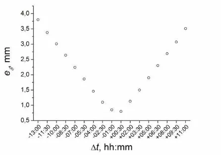
Following the procedure in (Wimmers and Velden, 2011) let us consider as a local measure of interpolation error the residual data δ in a given node, i.e. the absolute difference between the “actual” TPW value obtained from SSMIS F17 measurements and the closest in time interpolated TPW value originated from SSMIS F16 data. Let us assume then that the integral characteristic of the accuracy eδ is the average δ throughout the volume of the whole sample. In order to investigate the effect of spatiotemporal interpolation let us analyze eδ as a function of “proximity in time” Δtbetween “actual” and interpolated value, considering not only the minimal achievable Δt (about 30 minutes), but also other Δt values (with 1.5 hour step) within the daily interval.
The overall results of calculation of eδ as a function of Δt(Δt negative values correspond to the earlier times of interpolation compared to the time of SSMIS F17 measurements over the interpolation, also reaches its minimum of 0.8 mm.
Figure 1. Interpolation accuracy (circles) of TPW fields as function of time discrepancy, see Section 4
The described features of eδ are in good agreement with the results obtained in (Wimmers and Velden, 2011), and in particular, shown in Figure 8 of this work (not represented here). However, the final estimate of the accuracy in the cited paper is 0.5 - 2.0 mm. This is due to the fact that the algorithm implements a non-uniform temporal interpolation scheme: different portions of data must be “advected” through different time intervals in order to form a composite field coherent in time. Thus, the best accuracy of 0.5 mm is in fact not attainable for the most of the data because it reflects the residual errors in the source data from different sensors. When data requires some temporal interpolation this algorithm, according to Figure 8, gives an error ≥ 1.0 mm, and the error grows up to 2.0 mm as the algorithm attempts to compensate the time discrepancy of about 7 hours. Let us notice that a source to this error (in addition to those indicated by the authors) can partly reside in the approach to evaluate the displacement vector fields Vi. While in presented approach Vi are calculated directly from the source data, in (Wimmers and Velden, 2011) they are constructed as a weighted sum of wind fields (from ancillary numerical model) at a set of horizons. Such an approach implies a fixed vertical water vapor profile while it is not quite exact for complex atmospheric conditions over wide areas. However, the achieved accuracy is considered very reasonable for most applications.
5. ESTIMATION OF LATENT HEAT ADVECTION
When choosing TPW product as W fields the calculated Vi fields being geometrically calibrated and normalized (Ermakov et al, 2013a) have the sense of effective (integral by the height of the atmosphere) velocity of the water vapour advection. Calculated with the use of these velocity vectors flux of W through a given contour multiplied by a constant factor q = 2.26 MJ/kg has a sense of latent heat flux Q into or out of the area enclosed by the border with vertical sidewalls which projections on the Earth surface repeat the given contour.
For brevity let us give only the final expressions. If a displacement vector with the beginning at a node (x, y) has the coordinates (mx, my) on a regular grid with a step of s degrees, the corresponding velocity of advection is given by:
where R = 6371 km, radius of the Earth
Δt = time step of interpolation (1.5 or 3 hours).
Advective latent heat flux across an elementary border crossing the node (x, y) at some angle so that its normal has coordinates
where r = distance from border to observation point W(x, y) = TPW value at the node (x, y).
A “polar” representation of the flux through a given elementary border is especially useful for the case of circular contours when integration is carried out under fixed value of r for αfrom 0 through 2π. Consider an example in which established is a system of contours in the form of concentric circles of different radii, drifting along with the tropical cyclone (TC). In a number of cases studied (Ermakov et al, 2014) in the different basins of the World Ocean, when a TC eye is sufficiently distant from a coastline it is possible to identify an interrelation between the variations of TC intensity (maximum sustainable wind in the wall of the eye) and the advective latent heat flux, calculated as described in (Ermakov et al, 2013a).
Below considered are the two case studies carried out for the tropical cyclones of August, 2000, including hurricane Alberto, and those in November, 2013, including super typhoon Haiyan.
5.1 Case study: Tropical cyclones in August, 2000
For the interval of August, 2000 the most appropriate satellite due to the proximity of measurements in time (about 0.5 hour in August, 2000). F13 data (measured about 2.5 hours earlier than F14 data over the same region) were used sporadically to diminish few vast data gaps in absence of fast atmospheric motions.
The source data were spatiotemporally interpolated as described in Section 2 on the regular grid with 0.2° spatial step and 3-hour time sampling. A system of concentric circular contours of radii ranging from 2° to 8° was established. With the use of the interpolated TWP fields and displacement vector fields recalculated into velocity vectors the advective fluxes Q of latent heat through these contours were calculated, while at every 3-hour time step the system of contours was centered at the eye of the TC under investigation (a total of 7 TC all over the World Ocean were studied). In order to suppress possible positioning errors the system of contours was each time shifted one node (0.2°) in every direction, the corresponding values of Q were calculated for each radius. The resulting value was the average Q per every radius.
The estimates of the advective latent heat fluxes considered as functions of time were matched against the TC intensity (maximum sustainable wind) as function of time. The information on initial approximation of TC center as well as on TC intensity was extracted from the “Global-TC” database of IKI RAS (Pokrovskaya and Sharkov, 2006). The results of the investigation are discussed in the next section.
5.2 Case study: Tropical cyclones in November, 2013 For the interval of November, 2013 the most appropriate satellite microwave data were those provided by AMSR-2 onboard GCOM-W1 satellite and of SSMIS instruments on F16, and F17 satellites of DMSP series. In this case the ready TPW products were used as source data, namely RSS daily data products (separated by ascending/descending orbits) based on SSMIS data, and JAXA data products based on single AMSR-2 swaths. Temporal proximity of F16 nad F17 measurements was about 1 hour in November 2013, while the AMSR-2 measurements were 3.5 – 4.5 hours ahead. Due to this reason the advanced multisensory data processing scheme (see Section 3) was applied.
In the first processing stage the TWP fields based on SSMIS F16 data were supplemented with TWP fields from SSMIS F17 data and spatiotemporally interpolated on the regular grid with 0.25° spatial step and 1.5-hour time sampling (TPW SSMIS fields). AMSR-2 daily data (separately for ascending/descending swaths) were interpolated and merged on a regular grid with 0.125° spatial step. Then the interpolated TPW SSMIS fields closest in time to the local time of AMSR-2 measurements (attainable time discrepancy was about 0.5 hour) were used to supplement the AMSR-2 TWP fields in lacunae and other data gaps. To merge the data on a common grid the appropriate TPW SSMIS fields were additionally bi-linearly interpolated from 0.25° to 0.125° grid. The resulting TPW fields were spatiotemporally interpolated on the 0.125° grid with the time sampling of 1.5 hour.
The approach of the further estimations of latent heat fluxes Q and their combined analysis with intensity variations of tropical cyclones and tropical storms was principally similar to that described in paragraph 5.1. A minor difference was that the analysis was carried out with better spatiotemporal resolution. It was also supplemented with consideration of sea surface temperature (SST) along the TC tracks. To this end the RSS daily SST composites were used. For every position of a TC eye center along its track the average SST within a 1.5°-diameter circle one day before TC, one day after TC, and 3 days after TC were calculated, as well as their differences, and were analyzed as functions of time together with other characteristics (advective latent heat flux and TC intensity).
The main focus of investigation was the super typhoon Haiyan. Also considered was a tropical storm Podul which was generated several days after Haiyan and developed over similar ocean conditions but did not approach the typhoon stage. The results of the investigation are discussed in the next section.
6. DISCUSSION OF RESULTS 6.1 Tropical cyclones in August, 2000
Atlantics on 08/03 – 08/23 by a complex trajectory distant from coastlines and experienced three stages of rapid intensification.
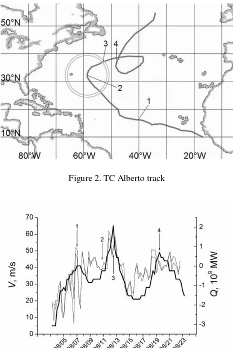
Figure 2 illustrates the TC Alberto track. Figure 3 demonstrates the evolution of its intensity V, m/s (thick line, left axis) together with the synchronized estimations of the advective latent heat flux Q, MW (thin lines, right axis) during the whole TC lifetime. Positive values of Q correspond to flux inside the contour (convergence). The enumerated arrows in Figures 2 and 3 indicate the same moments of time, namely the first intensity maximum (1), the beginning of the second intensification (2), the second intensity maximum (3) and the third intensity maximum (4). The fluxes Q shown in Figure 3 were calculated through the two circular contours of nearly the same radii of about 8° (shown in Figure 2) and plotted together in order to estimate the stability of calculations in respect to small changes of a contour.
Figure 2. TC Alberto track
Figure 3. TC Alberto evolution: here and further on thick line – TC intensity V; thin lines – advective latent heat fluxes Q
It can bee seen from Figure 3 that the estimations of Q is quite stable in respect to small changes of the contour of integration. The overall pattern of Q plots reflects remarkably well the evolution of TC intensity: positive values and increase of Q (convergence of latent heat) generally correspond to intensification of TC while negative values and decrease of Q correspond to dissipation of TC. It is also worth noting that the variations of Q are of order of several petawatts (109 MW) which correlates well with some estimates of maximum TC power (Ermakov et al, 2014).
The proximity to the coastline could possibly affect the estimates in the beginning of the TC Alberto trajectory (08/03 – 08/05). In order to demonstrate the influence of the coastline proximity let us consider another example: TC Ewiniar (08/11 – 08/18) which developed in the North-West Pacific and experienced two stages of rapid intensification, while the second half of its track lied in vicinity of the coastline of Japan, see Figure 4.
Figure 4. TC Ewiniar track
Figure 5. TC Ewiniar evolution, large contours for Q
Figure 6. TC Ewiniar evolution, small contours for Q
synchronized estimations of the advective latent heat flux Q, MW (thin lines, right axis) during the whole TC lifetime. The enumerated arrows in Figures 4, 5, and 6 indicate the same moments of time, namely the first intensity maximum (1), the dissipation phase (2), and the second intensity maximum (3).
The values of Q plotted in Figure 5 were calculated through the two circular contours of nearly the same radii of about 8° (shown in Figure 4 with thick gray circles). It can be seen that Q plots in Figures 5 can satisfactory reflect only the first intensity peak of the TC Ewiniar. The estimates for the second half of its track are significantly disturbed by the proximity of the coastline.
Due to the fact the TC Ewiniar was about twice less intense and smaller than the TC Alberto the reasonable estimates of Q can be obtained with the use of reduced radii of contours of integration. Those plotted in Figure 6 were calculated through the two circular contours of nearly the same radii of about 4° (shown in Figure 4 with thin black circles). It can be seen in Figure 6 that the pattern of Q plots has significantly changed in its right half and now reflects remarkably well both the first intensity peak and the maximum TC intensity on 08/15.
It should be noticed that the estimations are quite stable to small changes of the sizes of the contour of integration, and the variations of Q are again of the order of 109 MW though somewhat smaller than those calculated for the TC Alberto, especially in the case of reduced radii.
In sum all the hurricanes and typhoons of August, 2000 were analyzed in the same way, and principally the same behavior of Q plot patterns was observed (intensification of a TC corresponds to convergent latent heat flux, while dissipation corresponds to divergent one) in all cases wherever the coastlines did not disturb significantly the results of the estimations (Ermakov et al, 2014).
6.2 Tropical cyclones in November, 2013
Among tropical cyclones of November, 2013 the super typhoon Hiayan is of great interest (Mori et al, 2014). It was formed in the North West Pacific and evolved over the deeply warmed ocean (Lin et al, 2014) on 11/02 – 11/11 moving quickly ashore by almost straight westward trajectory. The fast drift of Haiyan is believed to determine (along with appropriate ocean conditions) extreme characteristics of Haiyan (Lin et al, 2014) due to smaller cooling effect. However this also means that the ocean conditions remained almost undisturbed by Haiyan which is also proved by the absence of a cold trail and significant sea surface temperature (SST) anomalies in the next days (see below). Nevertheless the next several tropical storms (TS) including TS Podul generated a week after Haiyan in the same region and travelling in almost the same direction but somewhat to the south off the Haiyan track on 11/09 – 11/15 were not even close to evolve into a super typhoon. Figure 7 illustrates the tracks of the TC Haiyan and the TS Podul.
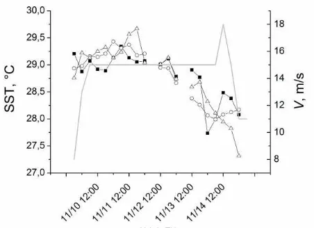
Figure 8 demonstrates SST measured along the TC Haiyan track one day before (black squares), one day after (open circles), and 3 days after (open triangles) the TC passed corresponding areas (see paragraph 5.2) together with the TC intensity, V (thick gray line, right axis). The same quantities for TS Podul track are plotted in Figure 9. It can be seen that SST was not affected significantly by both Haiyan and Podul, varying in almost the same range with maximum of 29.7 - 30°C, and its temporal
variations all along the considered tracks were less than 1°C, both negative and positive.
Figure 7. Tracks of the TC Haiyan (H) and the TS Podul (P)
Figure 8. SST along TC Haiyan track (marked lines) and the TC intensity (thick gray line), see paragraph 6.2 for details
Figure 9. SST along TS Podul track (marked lines) and the TS intensity (thick gray line), see paragraph 6.2 for details
same quantities for TS Podul. The smaller contours of 4° radii were used due to vicinity of the coastline and much smaller intensity of the TS.
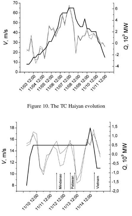
Figure 10. The TC Haiyan evolution
Figure 11. The TS Podul evolution
It can be seen from these figures that the Q plots in both cases reflect quite well the intensity variations of the TC Haiyan and the TS Podul. The rapid intensification of the former corresponds to significant increase of Q up to 6 PW. On the contrary in the case of the TS Podul the Q plot oscillates around 0 with the amplitude less than 1 PW, falling down significantly each time when the TS crosses coastlines (indicated with arrows and toponym in Figure 11). This corresponds well to almost unchanged intensity of the TS of about 15 m/s. Hence, both cases prove the same concept formulated in paragraph 6.1: a TC intensity is found to be interrelated with the advection of heat flux, calculated through the contour that surrounds the TC wall: increase of a TC intensity corresponds to positive (convergent) flux, while its decrease corresponds to negative (divergent) one. This flux can be estimated with the use of the described calculation scheme closed in respect to the satellite microwave data.
7. CONCLUSIONS
The approach of satellite radiothermovision is presented which consists of a set of processing techniques applicable for multisource data of passive microwave monitoring of ocean-atmosphere system, and allows creating dynamic description of
mesoscale and synoptic atmospheric processes and estimating physically meaningful integral characteristics of the observed processes (like avdective flow of the latent heat through a given border).
The approach is demonstrated on a case study of tropical cyclones of August, 2000, and November, 2013. The investigation reveals a remarkable interrelation between the intensity of a TC and the estimate of advective latent heat flux through a contour surrounding the TC: convergent flux corresponds to the TC intensification while divergent flux corresponds to its dissipation. This interrelation requires more thorough examination on a large number of tropical cyclones travelling distantly enough from coastlines.
However the presented approach opens wider opportunities for a researcher. One of those is a combined analysis of a set of geophysical parameters interpolated to a common grid and “synchronized” on a timeline with a good accuracy (one hour and less). Other interesting opportunity is to consider different types of contours and borders to investigate latent heat flux and other integral characteristics. For example introducing a system of borders lying along the parallels at different latitudes one can study the process of polar transport over the selected basin or the whole World Ocean.
One of the advantages of the presented approach is that the calculation scheme is closed in respect to the satellite microwave data, hence, conceptually simplifies the analysis by requiring no additional information to be gathered and processed.
ACKNOWLEDGEMENTS
The SSMIS data used for the preparation on this paper are produced by Remote Sensing Systems and sponsored by the NASA Earth Science MEaSUREs Program and are available at www.remss.com. AMSR2 data used for the preparation of this paper was supplied by the GCOM-W1 Data Providing service, Japan Aerospace Exploration Agency. The design of the specific data processing software used to process the satellite data products was partly supported by RFBR grant N15-07-04422.
REFERENCES
Ermakov D.M., Raev M.D., Suslov A.I. and Sharkov E.A., 2007. Electronic long-standing database for the global radiothermal field of the Earth in context of multi-scale investigation of the atmosphere-ocean system. Issledovanie Zemli iz Kosmosa, 1, pp. 7-13. (in Russian)
Ermakov, D.M., Chernushich, A.P., Sharkov, E.A. and Shramkov, Ya.N., 2011. Stream Handler system: an experience of application to investigation of global tropical cyclogenesis. Proceedings of ISRSE-34, Sydney, Australia
http://www.isprs.org/proceedings/2011/ISRSE-34/211104015Final00456.pdf (24 Feb. 2015)
Ermakov, D.M., Chernushich A.P., Sharkov E.A. and Pokrovskaya I.V., 2013b. Searching for an energy source of the intensification of tropical cyclone Katrina using microwave satellite sensing data. Izvestiya, Atmospheric and Oceanic Physics, 49(9), pp. 963-973.
Ermakov, D.M., Raev M.D., Chernushich A.P. and Sharkov E.A., 2013c. An algorithm for construction global ocean-atmosphere radiothermal fields with high spatiotemporal sampling by satellite microwave measurements. Issledovanie Zemli iz Kosmosa, (Earth Research from Space), 4, pp. 72-82. (in Russian)
Ermakov, D.M., Sharkov E.A., Pokrovskaya I.V. and Chernushich A.P., 2013d. Revealing the energy sources of alternating intensity regimes of the evolving Alberto tropical cyclone using microwave satellite sensing data Izvestiya, Atmospheric and Oceanic Physics, 49(9), pp. 974-985.
Ermakov, D.M., Sharkov E.A. and Chernushich A.P., 2014. The role of tropospheric advection of latent heat in the investigation of tropical cyclones. Issledovanie Zemli iz Kosmosa, (Earth Research from Space), 4, pp. 3-15. (in Russian)
Lin, I.-I., Pun, I.-F. and Lien, C.-C., 2014. “Category-6” supertyphoon Haiyan in global warming hiatus: Contribution from subsurface ocean warming. Geophysical Research Letters, 41(23), pp. 8547-8553.
Mori, N., Kato, M., Kim, S., Mase H., Shibutani, Y., Takemi, T., Tsuboki, K. and Yasuda, T., 2014. Local amplification of storm surge by Super Typhoon Haiyan in Leyte Gulf. Geophysical Research Letters, 41(14), pp. 5106-5113.
Nerushev, A.F. and Kramchaninova, E.K., 2011. Method for determining atmospheric motion characteristics using measurements on geostationary meteorological satellites. Izvestiya, Atmospheric and Oceanic Physics, 47(9), pp. 1104-1113.
Pokrovskaya I.V. and Sharkov E.A., 2006. Tropical cyclones and tropical disturbances of the World Ocean: chronology and evolution. Version 3.1 (1983 – 2005). Poligraph servis, Moscow, 728 p.
Richardson, I.E.G., 2003. H.264 and MPEG-4 video compression. John Wiley & Sons Ltd, The Atrium, Southern Gate, Chichester, West Sussex PO19 SQ, England. 306 p.
Ruprecht, E., 1996. Atmospheric water vapor and cloud water: an overview. Advances in Space Research, 18(7), pp. 5-16.
Wentz, F.J., 1997. A well-calibrated ocean algorithm for SSM/I. Journal of Geophysical Research, 102(C4), pp. 8703-8718.