8 Transportation Research Record: Journal of the Transportation Research Board, No. 2482, Transportation Research Board, Washington, D.C., 2015, pp. 8–15. DOI: 10.3141/2482-02
Heavy-duty diesel maintenance equipment consumes significant amounts of fuel and consequently emits substantial quantities of pollutants. The purpose of this study was to identify which engine activity variables had the greatest impact on fuel use and emissions rates. A real-world data set was used for a case study fleet containing backhoes, motor graders, and wheel loaders. Multiple linear regression was used to assess the relation-ships between engine activity variables and fuel use and emissions rates. The engine activity variables of engine speed, manifold absolute pres-sure, and intake air temperature were used to predict mass per time fuel use and emissions rates of nitrogen oxides, hydrocarbons, carbon monoxide, carbon dioxide, and particulate matter. The results indicated that manifold absolute pressure had the greatest impact on fuel use and emissions rate predictions. Based on this finding, fuel use and emissions estimating models based on manifold absolute pressure were developed as a practical estimating tool for practitioners.
Highway maintenance activities are a major part of infrastructure asset management. Many of these activities are performed by heavy-duty diesel (HDD) equipment. This equipment consumes large quan-tities of diesel fuel and thus emits large quanquan-tities of pollutants and greenhouse gases (GHGs). The energy and environmental impacts of these activities and equipment are significant.
Fleet managers have long been able to estimate their required fuel consumption based on historical records. Because of drastic price increases in recent years, it is now more important than ever to be able to estimate future fuel requirements to manage infrastructure maintenance costs. Furthermore, most fleet managers seldom con-cern themselves with the environmental impact of their equipment, specifically air pollutant emissions. As new environmental regulations appear on the horizon, fleet managers can no longer afford to disregard the energy and environmental impacts of their work. They must be able to quantify the fuel use and emissions of their equipment to manage them.
The objective of this study was to establish a modeling frame-work for estimating fuel use and emissions of HDD equipment used for highway maintenance activities. To do so, it was necessary to
understand equipment activity, especially engine performance. The primary research question was: Which engine variables have the greatest impact on fuel use and pollutant emissions rates for HDD equipment?
BACKGROUND
According to the U.S. Environmental Protection Agency (EPA), there are approximately two million items of off-road HDD construction and mining equipment in the United States (1). This equipment con-sumes about six billion gal of diesel fuel annually. EPA also estimates that in 2005, HDD construction equipment emitted approximately 657,000 tons of nitrogen oxides (NOx), 1,100,000 tons of carbon monoxide (CO), and 63,000 tons of particulate matter (PM). Each of these pollutants is a criteria pollutant as designated by the EPA National Ambient Air Quality Standards (NAAQS) (2). Other pollut-ants found in diesel exhaust include hydrocarbons (HCs), which are a precursor to ground-level ozone (another NAAQS criteria pollutant). Although not a regulated pollutant, carbon dioxide (CO2) is perhaps the most recognized emission from HDD equipment because of its notoriety as a GHG and its potential global warming effect.
Diesel emissions have many impacts on human health and the environment. Diesel exhaust may lead to serious health conditions, including asthma and allergies, and can worsen heart and lung disease, especially in vulnerable populations like children and the elderly. PM and NOx emissions lead to the formation of smog and acid rain, which damage plants, animals, crops, and water resources. CO2 is a major GHG emission that leads to climate change, which affects air quality, weather patterns, sea level, ecosystems, and agriculture. Reducing GHG emissions from diesel engines through improved fuel economy and idle reduction strategies can help address climate change, improve the nation’s energy security, and strengthen the economy. Another concern with diesel emissions is environmental justice. It is possible that many minority and dis-advantaged populations may receive disproportionate impacts from diesel emissions (3).
To quantify and characterize HDD emissions, reliable prediction models are needed; however, most fuel use and emissions predic-tion tools are based on engine dynamometer data. Although engine dynamometer testing is a reliable source of data, it is performed in a laboratory setting and does not accurately represent the episodic nature of real-world equipment activity. The data used for the modeling efforts presented in this paper are based on real-world data collected from in-use HDD equipment by an on-board portable emissions measurement system (PEMS).
Engine Variable Impact Analysis of
Fuel Use and Emissions for Heavy-Duty
Diesel Maintenance Equipment
Phil Lewis, Heni Fitriani, and Ingrid Arocho
SCOPE
The equipment of interest for this study included backhoes, motor graders, and wheel loaders. These types of equipment were selected because they are often used for many highway maintenance activities and are frequently the most represented units in a highway mainte-nance fleet. The case study equipment was owned by either the North Carolina Department of Transportation or private fleet owners in the Raleigh, North Carolina, area. The equipment was observed perform-ing activities such as light gradperform-ing, fine gradperform-ing, excavatperform-ing, and hauling materials.
The HDD equipment engine activity variables include measure-ments of engine speed in revolutions per minute (rpm), manifold absolute pressure (MAP), and intake air temperature (IAT). The pollutant measurements include NOx, HC, CO, CO2, and PM. Fuel use measurements were also collected. The engine activity variables were used to predict fuel use and emissions rates.
PREVIOUS WORK
The most prominent and well-documented data set of real-world fuel use and emissions measurements from off-road HDD equipment was developed by researchers at North Carolina State University from 2005 through 2008. This data set is widely considered to be the largest publicly available source of real-world fuel use and emissions data for nonroad construction equipment. The research team utilized PEMS testing to collect, analyze, and characterize real-world engine, fuel use, and emissions data from more than 30 items of HDD equipment. The equipment types included back-hoes, bulldozers, excavators, motor graders, off-road trucks, track loaders, and wheel loaders. For some of the equipment, the team made comparisons of pollutant emissions for petroleum diesel versus those for B20 biodiesel.
Many papers have been published based on the aforementioned data set. Lewis et al. outlined requirements and incentives for reducing air pollutant emissions from construction equipment (4). The authors also compared sources of emissions from various types of equipment. On the basis of those concepts, Lewis et al. devel-oped a fuel use and emissions inventory for a publicly-owned fleet of nonroad diesel construction equipment (5). This emissions inven-tory quantified emissions of NOx, HC, CO, and PM for the fleet for petroleum diesel and B20 biodiesel. The results were categorized by equipment type and EPA engine tier standards. The impacts on the inventory of different emissions reduction strategies were com-pared. Frey et al. followed up this work by presenting the results of a comprehensive field study that characterized and quantified real-world emissions rates of NOx, HC, CO, and PM from nonroad diesel construction equipment (6). Average emissions rates were developed for each equipment type and were presented on a mass per time basis and mass per fuel used basis for petroleum diesel and B20 biodiesel. Frey et al. conducted a comparison of B20 versus petroleum diesel emissions for backhoes, motor graders, and wheel loaders working under real-world conditions (7). Frey et al. also com-pared emissions rates for the different EPA engine tier standards of the equipment.
Lewis et al. published a series of papers on the impacts of idling on equipment fuel use and emissions rates (8–10). These papers quanti-fied the change in total activity fuel use and emissions as the ratio of idle time to non-idle time changes. The major finding was that total fuel use and emissions for an activity increase as equipment idle
time increases. Ahn et al. used the data set and previous studies to develop an integrated framework for estimating, benchmarking, and monitoring pollutant emissions from construction activities (11). Hajji and Lewis developed a productivity-based estimating tool for fuel use and air pollutant emissions for nonroad construction equip-ment performing earthwork activities (12). The methodology for the field data collection in these studies used a PEMS and is well documented by Rasdorf et al. (13). Frey et al. also outlined the meth-ods and procedures for collecting and analyzing data for construction equipment activity, fuel use, and emissions; thus, the methodology may be easily duplicated by those with the necessary expertise and implementation (14, 15).
METHODOLOGY
This section addresses the research approach that was used to evaluate the impact of engine activity parameters on the fuel use and emissions rates of HDD maintenance equipment. The data set used to conduct the analysis is described. The modeling methods used to define the relationships between engine activity and emissions data are pre-sented. The approach for evaluating the impact of each engine activity variable on fuel use and emission rates is provided.
Engine Activity and Emissions Data
The data used in this paper were based on real-world data sets developed by North Carolina State University. Data were collected from 31 items of HDD equipment, including five backhoes, six bull-dozers, three excavators, six motor graders, three off-road trucks, three track loaders, and five wheel loaders. The focus of this study was HDD equipment typically used for highway maintenance; therefore, five backhoes, six motor graders, and five wheel loaders were examined.
The real-world data sets included second-by-second measure-ments of engine activity parameters and emissions data. The engine activity data included RPM (rpm), MAP (kPa), and IAT (°C). These are common engine activity variables that are generally measurable for all types of vehicles. It should be noted, however, that the PEMS subset of instruments for measuring engine activity was limited to these three variables. Although more recently manufactured nonroad equipment may have an onboard diagnostics system that records values for these variables (as well as others) via a PEMS interface, the data used in this study were collected directly from the engine by specialized PEMS instrumentation.
The emissions data included mass per time (g/s) rates of NOx, HC, CO, CO2, and PM. Mass per time (g/s) fuel use measurements were also collected. All these data were collected simultaneously and on the same timescale (s) as the engine activity data; thus, it was possible to identify relationships between the engine activity, fuel use, and emissions for each item of equipment. In the analysis presented here, fuel use and emissions were dependent variables and engine activity parameters were independent variables.
Multiple Linear Regression Models
The dependent (or response) variables included mass per time fuel use rates and emission rates of NOx, HC, CO, CO2, and PM; hence, six MLR models were developed for each item of equipment. The MLR equations for fuel use and emission rates for each pollutant had the following form:
Y1 6− = β + β0 1X1+ β2X2+ β3X3 (1)
where
Y1–6 = fuel use or emissions rate of NOx, HC, CO, CO2, or PM (g/s);
X1 = MAP (kPa);
X2 = engine speed (rpm);
X3 = intake air temperature (°C); and
β0, β1, β2, β3 = coefficients of linear relationship.
A forward stepwise variable selection method was used to develop the MLR models. The criteria to include a variable in the model were based on probability (p-values). If the p-value of the variable was less than .05, the variable was included in the model. Conversely, if the p-value was greater than .05, the variable was not included in the model. The analysis of variance and analysis of maximum likelihood for each response variable were also conducted. The conditions of the MLR models were investigated with residual plots, including the normal probability plot of the residuals, residuals versus the fitted values, histogram of the residuals, and residuals versus the order of data.
Variable Impact Analysis
The purpose of variable impact analysis (VIA) is to measure the sensitivity of prediction models to changes in independent vari-ables (16). As a result of the analysis, every independent variable is assigned a relative variable impact value. These are percentage values and sum to 100%. The lower the percentage value for a given variable, the less impact the variable has on the predictions. The results of the analysis help in the selection of a new set of independent variables, possibly a set that will enable more accurate predictions. For example,
a variable with a low impact value can be eliminated in favor of a new variable.
The results of VIA are relative to a given set of models; thus, if one variable is disregarded in a set of models, that does not mean that it will not be of value to another set of models for making a significant contribution to accurate predictions. In data sets with smaller numbers of cases or larger numbers of variables, the differ-ences in the relative impacts of the variables between sets of models may be more pronounced. For example, consider a model with two independent variables in which one is assigned 99% and the other 1%. This assignment means that the latter is much less important than the former, but it does not mean that the latter is unimportant altogether, particularly if high accuracy of predictions is desired.
VIA is not intended to support firm conclusions such as stating with high confidence that a given variable is irrelevant. Instead, the intention is to aid in a search for the best set of independent variables. The results of VIA may suggest that a given variable looks irrelevant, sufficiently so that it may be worthwhile to develop models without this variable. In this study, VIA was used to determine the relative impact of RPM, MAP, and IAT on predicting fuel use and emissions rates of NOx, HC, CO, CO2, and PM.
RESULTS
This section presents the results of the VIA. A data collection summary of the case study equipment is presented. A summary of the precision of the MLR models is provided. The engine vari-ables that had the highest impact on fuel use and emissions rates are identified.
Engine Activity and Emissions Data
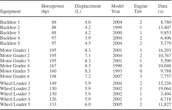
Table 1 summarizes the HDD equipment specifications and the quantity of data that was collected for each item of equipment. Engine tier refers to the EPA regulation imposed on engine manufactur-ers, which is aimed at reducing emissions rates of NOx, HC, CO, and PM. Almost half the units tested were Tier 1. The horsepower
TABLE 1 HDD Equipment Specifications and Data Collection
Equipment
Horsepower (hp)
Displacement (L)
Model Year
Engine Tier
Data (s)
Backhoe 1 88 4.0 2004 2 8,780
Backhoe 2 88 4.2 1999 1 13,407
Backhoe 3 88 4.2 2000 1 9,853
Backhoe 4 97 3.9 2004 2 6,406
Backhoe 5 97 4.5 2004 2 5,379
Motor Grader 1 195 8.3 2001 1 16,293
Motor Grader 2 195 7.1 2004 2 10,767
Motor Grader 3 195 8.3 2001 1 5,590
Motor Grader 4 167 8.3 1990 0 10,040
Motor Grader 5 160 8.3 1993 0 9,788
Motor Grader 6 198 7.2 2007 3 7,757
Wheel Loader 1 149 5.9 2004 2 15,226
Wheel Loader 2 130 5.9 2002 1 19,064
Wheel Loader 3 130 5.9 2002 1 3,404
Wheel Loader 4 126 5.9 2002 1 6,718
rating and displacement values were quantitatively similar for all items in a particular equipment type. The model years ranged from 1990 (Motor Grader 4) to 2007 (Motor Grader 6). Overall, almost 45 h of data were collected for the case study equipment. This total included approximately 12 h for backhoes, 17 h for motor graders, and 16 h for wheel loaders.
Table 2 summarizes the average values of engine activity, fuel use, and emissions for each of the equipment units in the case study fleet. The purpose of this table is to show the magnitude of the real-world data values that were collected. In the table, the equipment types with the highest average MAP and RPM also have the highest average fuel use and emissions rates. Furthermore, these equipment types also have the highest horsepower ratings and displacement values. Based on the data in Table 2, IAT appears to have little to no influence on fuel use and emissions rates, since backhoes had the highest aver-age IAT but the lowest averaver-age fuel use and emissions rates. Overall, motor graders have the highest average engine activity, fuel use, and emission rates, followed by wheel loaders and backhoes. This find-ing appears to support the intuitive conclusion that equipment with larger engines tend to consume more fuel and emit more pollutants on a mass per time basis.
MLR Models
MLR models were developed for each item of equipment, with fuel use, NOx, HC, CO, CO2, and PM as dependent variables and MAP, RPM, and IAT as independent variables. Overall, 96 MLR models were developed (6 dependent variables times 16 items of equipment). The variables MAP, RPM, and IAT were included in all the models based on the statistical significance test of p < .05. All p-values were much less than .01. This means that there is much less than a 1% probability that the coefficient assigned to the vari-able occurred randomly or by chance. A review of the residual plots indicated no problems or cause for concern with the conditions of the models. The MLR models, therefore, were considered reliable for conducting the VIA.
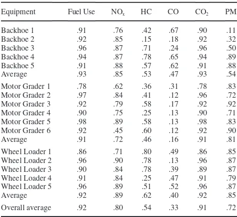
Table 3 summarizes the R2
values for the MLR models for each item of equipment in the case study fleet. The R2 value is a measure of precision for MLR models and has a range of 0 to 1. R2
equates to the percentage of variability in the data that is accounted for by the model. For example, the fuel use model for Backhoe 1 has a value of R2= .91. This means that approximately 91% of the variability in the fuel use data is accounted for by the model with MAP, RPM, and IAT. Overall, the MLR models accounted for a high percentage of the variability in the data for fuel use, NOx, CO2, and PM. The MLR models accounted for a moderate percentage of variability for HC and a comparatively low percentage of variability for CO; thus, it is reasonable to conclude that HC and CO are more difficult TABLE 2 Summary of Average Values for Engine Activity, Fuel Use, and Emissions
Equipment
Backhoe 1 104 905 20 0.43 0.02 0.000 0.000 1.3 0.02
Backhoe 2 101 1,256 26 0.93 0.03 0.003 0.009 2.9 0.30
Backhoe 3 104 1,225 56 0.74 0.02 0.002 0.004 2.3 0.35
Backhoe 4 112 1,119 51 0.41 0.02 0.002 0.001 1.3 0.09
Backhoe 5 111 1,095 47 0.42 0.02 0.002 0.003 1.3 0.11
Average 106 1,120 40 0.58 0.02 0.002 0.003 1.8 0.17
Motor Grader 1 174 1,789 30 4.8 0.18 0.015 0.02 15 1.40 Motor Grader 2 115 1,167 45 1.5 0.05 0.014 0.01 4.7 0.27 Motor Grader 3 149 1,746 41 2.2 0.08 0.042 0.01 7.0 0.78 Motor Grader 4 113 1,827 0 2.5 0.16 0.032 0.04 8.0 0.63 Motor Grader 5 120 1,405 12 2.3 0.12 0.014 0.05 9.9 0.53 Motor Grader 6 169 1,839 60 2.2 0.04 0.010 0.01 10 0.51
Average 140 1,628 31 2.6 0.11 0.021 0.02 9.1 0.68
Wheel Loader 1 122 1,217 30 1.5 0.05 0.012 0.02 4.8 0.42 Wheel Loader 2 118 1,373 21 1.4 0.05 0.002 0.01 4.3 0.41 Wheel Loader 3 119 1,192 19 0.8 0.04 0.002 0.05 2.6 0.12 Wheel Loader 4 126 1,392 18 1.0 0.04 0.004 0.00 3.2 0.31 Wheel Loader 5 105 1,072 33 0.7 0.22 0.002 0.01 2.2 0.13
Average 118 1,249 24 1.1 0.08 0.004 0.02 3.4 0.28
TABLE 3 Summary of R2 Values for MLR Models
Equipment Fuel Use NOx HC CO CO2 PM
Backhoe 1 .91 .76 .42 .67 .90 .11
to predict than fuel use, NOx, CO2, and PM when MAP, RPM, and IAT are used as predictor variables.
Variable Impact Analysis
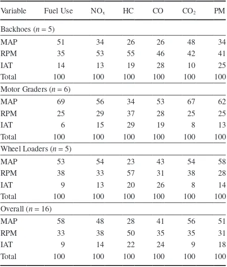
Table 4 presents the average engine variable impact for each depen-dent variable and each item of equipment. On the basis of overall aver-ages, and in most cases the equipment type averaver-ages, MAP has the greatest impact on predictions of fuel use, NOx, CO, CO2, and PM. The variable RPM has the next highest average impact on these dependent variables. For HC, RPM has the greatest average impact, followed by MAP. IAT has the least average impact of any of the independent variables on all the dependent variables. This does not mean that IAT has no predictive power and should be disregarded in future models. It means only that IAT does not have as much influence on fuel use, NOx, HC, CO, CO2, and PM relative to MAP and RPM.
Simplified Approach to Estimating Fuel Use and Emissions
One of the intended purposes of VIA is to select a subset of variables that may produce accurate models. Based on the results of the VIA, a set of simple models that use one independent variable were inves-tigated for predicting fuel use and emissions for HDD equipment. Since MAP had the greatest overall impact on fuel use and emis-sions, it was a logical candidate for a predictor variable for the new models. The variable MAP varies with engine load in turbocharged engines (all engines in the case study fleet were turbocharged); thus, MAP is a good surrogate for engine load. Furthermore, engine load
is much easier to estimate compared with RPM and IAT for a given activity. Many construction equipment textbooks and equipment performance handbooks use engine load as a basis for fuel use esti-mating equations (17–20); therefore, MAP as a surrogate for engine load was selected to develop the new, simplified models.
Since measurements of MAP vary among individual items of equipment, the MAP data were normalized according to Equation 2 to provide a common basis for selecting MAP-based engine load esti-mates. The normalized MAP values range from 0% to 100%, simi-larly to engine load estimates, and are easier to estimate compared with actual MAP values measured in kPa. In this case, a normalized MAP-based engine load estimate of 0% indicates the lowest engine load possible, such as equipment idling; an estimate of 100% represents the highest possible engine load, such as equipment operating at full throttle under adverse conditions.
Simple linear regression (SLR) models were developed that use normalized MAP values (as surrogates for engine load) to predict fuel use and emissions for each item of equipment in the case study fleet. SLR models employ one independent variable to predict a dependent variable. These models take the form shown in Equation 3:
Y1 6− =mX+b (3)
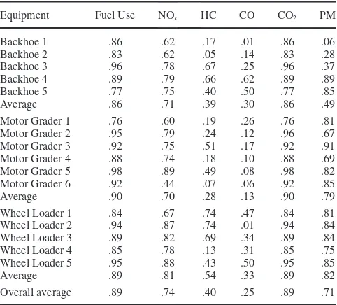
values for the SLR models for each item of equipment in the case study fleet. Compared with the MLR models in Table 3, which use three predictor variables, these simple one-variable models account for only slightly less variability in the data. On average, the SLR models have R2 values that are about 6% lower than those of the MLR models; therefore, the SLR models provide reasonable estimates for fuel use and emissions of NOx, HC, CO2, and PM on the basis of engine load. Although the models for HC and CO have more variability, they still provide adequate rough order of magnitude estimates for these pollutants.
The SLR models have the potential to be useful estimating tools for practitioners. Table 6 presents a summary of the models for fuel use and emissions in commonly used units: gal/h for fuel use; lb/h for emissions rates of NOx, HC, CO, and CO2; and g/h for PM. Further-more, these models were categorized on the basis of EPA engine tier standards. This categorization was accomplished by averaging the model coefficients for the items of equipment found in each engine tier. Tier 0 includes Motor Graders 4 and 5. Tier 1 includes Backhoes 2 and 3; Motor Graders 1 and 3; and Wheel Loaders 2, 3, and 4. Tier 2 includes Backhoes 1, 4, and 5; Motor Grader 2; and Wheel Loaders 1 and 5. This is an acceptable approach because the TABLE 4 Average Engine Variable Impact
for Each Equipment Type (%)
Variable Fuel Use NOx HC CO CO2 PM
Backhoes (n= 5)
MAP 51 34 26 26 48 34
RPM 35 53 55 46 42 41
IAT 14 13 19 28 10 25
Total 100 100 100 100 100 100
Motor Graders (n= 6)
MAP 69 56 34 53 67 62
RPM 25 29 37 28 25 25
IAT 6 15 29 19 8 13
Total 100 100 100 100 100 100
Wheel Loaders (n= 5)
MAP 53 54 23 43 54 58
RPM 38 33 57 31 38 28
IAT 9 13 20 26 8 14
Total 100 100 100 100 100 100
Overall (n= 16)
MAP 58 48 28 41 56 51
RPM 33 38 50 35 35 31
IAT 9 14 22 24 9 18
engines are designed to meet specific EPA engine tier emissions standards rather than being designed for a particular type of equip-ment or activity. As anticipated, the fuel use and emissions estimates decrease as engine tier increases, although there is little difference in the models for HC and CO. These pollutants are difficult to model precisely because of their high variability in the original field data.
To assist practitioners further with estimating fuel use and emis-sions, Figure 1 presents a cumulative frequency diagram of engine load versus time for backhoes, motor graders, and wheel loaders. The figure was developed by summing the amount of time that each item of equipment spent in each range of normalized MAP. Since the equipment is designed to accommodate particular types of activities, engine load versus time was categorized by equipment type and not EPA engine tier. Figure 1 shows the average engine load versus time for each equipment type. The figure represents the cumulative time, on average, that each equipment type spends at or below a specific engine load. For example, backhoes and wheel loaders spend approximately 60% of their work time at an engine load of 20% or less; thus, more than half their work time is spent
at low engine loads. Motor graders spend approximately 60% of their time at or below an engine load of 50%, which is much higher compared with backhoes and wheel loaders. Figure 1 provides a useful guide for practitioners to estimate probable engine loads as the predictor variable for the SLR models.
CONCLUSIONS
The primary research question for this paper was: Which engine variables have the greatest impact on fuel use and emission rates for HDD equipment, particularly backhoes, motor graders, and wheel loaders? This question was investigated through a rigorous statistical analysis based on real-world engine activity, fuel use, and emissions data. The following are the conclusions of this analytical effort:
• MAP, followed by RPM, has the greatest impact on mass per time rates of fuel use, NOx, CO, CO2, and PM.
• RPM, followed by MAP, has the greatest impact on mass per time rates of HC.
• IAT has the least impact on mass per time rates of fuel use, NOx, HC, CO, CO2, and PM.
The objective of this study was to establish a modeling frame-work for estimating fuel use and emissions of HDD equipment used for highway maintenance activities. This framework was accom-plished with the results of the VIA to determine which engine vari-able had the greatest influence on fuel use and emissions. With normalized MAP data as a surrogate for engine load, a set of simple one-variable models was developed to predict fuel use and pollutant emissions of NOx, HC, CO, CO2, and PM. To make the models more applicable, they were categorized according to EPA engine tier stan-dards. These models provide a practical and statistically defensible fuel use and emissions estimating tool for backhoes, motor graders, and wheel loaders.
Another key finding of this research effort is that HC and CO are difficult to predict because of high variability in the data. Although the MLR and SLR models accounted for small percentages of the variability in the real-world data, the models still provide at least a rough order of magnitude estimate for these pollutants. Conversely, TABLE 5 Summary of R2 Values for SLR Models
Equipment Fuel Use NOx HC CO CO2 PM
Backhoe 1 .86 .62 .17 .01 .86 .06
Backhoe 2 .83 .62 .05 .14 .83 .28
Backhoe 3 .96 .78 .67 .25 .96 .37
Backhoe 4 .89 .79 .66 .62 .89 .89
Backhoe 5 .77 .75 .40 .50 .77 .85
Average .86 .71 .39 .30 .86 .49
Motor Grader 1 .76 .60 .19 .26 .76 .81 Motor Grader 2 .95 .79 .24 .12 .96 .67 Motor Grader 3 .92 .75 .51 .17 .92 .91 Motor Grader 4 .88 .74 .18 .10 .88 .69 Motor Grader 5 .98 .89 .49 .08 .98 .82 Motor Grader 6 .92 .44 .07 .06 .92 .85
Average .90 .70 .28 .13 .90 .79
Wheel Loader 1 .84 .67 .74 .47 .84 .81 Wheel Loader 2 .94 .87 .74 .01 .94 .84 Wheel Loader 3 .89 .82 .69 .34 .89 .84 Wheel Loader 4 .85 .78 .13 .31 .85 .75 Wheel Loader 5 .95 .88 .43 .50 .95 .85
Average .89 .81 .54 .33 .89 .82
Overall average .89 .74 .40 .25 .89 .71
TABLE 6 Summary of SLR Models
Tier 0 Tier 1 Tier 2
Output m b m b m b
Fuel use (gal/h) 10 0.4 5.4 0.3 4.9 0.4
NOx (lb/h) 3.8 0.2 1.2 0.2 0.9 0.9
HC (lb/h) 0.2 0.1 0.2 0.0 0.1 0.0
CO (lb/h) 0.2 0.2 0.1 0.0 0.1 0.0
CO2 (lb/h) 225 8.0 120 6.0 110 8.0
PM (g/h) 8.8 0.3 5.3 0.3 3.3 0.2
NOTE: The values in the columns are for the following equation: Y=mX+b, where X= engine load, m= slope of regression line, and b=y-intercept.
0 20 40 60 80 100
0 20 40 60 80 100
Engine Load (%)
Time (%)
Backhoes Motor graders
Wheel loaders
fuel use rates and emission rates of NOx, CO2, and PM are quite predictable, especially as a function of MAP.
RECOMMENDATIONS
The results presented in this paper are limited to backhoes, motor graders, and wheel loaders. Although these items of equipment are prominent in most highway maintenance fleets, many other types of equipment should be included in the analysis. The study effort presented here should be expanded to include the other equipment types found in the real-world data sets, including bulldozers, exca-vators, off-road trucks, and track loaders. These equipment types may also be used in highway maintenance activities, but they are especially critical for general construction and earthwork tasks. Furthermore, the real-world data set should be updated to include Tier 3 and Tier 4 equipment as well as other equipment types such as cranes, scrapers, and tractors.
The analysis of the engine activity data was limited to MAP, RPM, and IAT. The data for those variables should be examined more closely to determine their true influence on fuel use and emissions. For example, previous studies mentioned in the literature review have shown that MAP and RPM are frequently highly correlated with each other; thus, multicollinearity may be a concern (6, 7, 14, 15). When this occurs, the coefficient estimates of the MLR models may change erratically in response to small changes in the model or the data. Multicollinearity does not reduce the predictive power or reliability of the model, but it does affect calculations regarding the individual predictor variables. In this case, MLR models with cor-related predictors can indicate how well MAP, RPM, and IAT predict fuel use and emissions, but they may not give valid results about any individual predictor, such as RPM, or about which predictor variables are redundant with respect to others. Furthermore, other equipment variables, such as engine horsepower and gross vehicle weight, may help provide higher-resolution results for fuel use and emissions estimating efforts.
The results of the study have shown that mass per time fuel use and emission rates are highly sensitive to MAP, which may be treated as a surrogate for engine load. Previous work highlighted in the literature review has shown that mass per fuel used emissions rates have less variability than mass per time emissions rates (6, 7, 14, 15). The mass per time emissions rates may be converted to mass per fuel used emissions rates by dividing them by the corresponding fuel use rate (lb/hr ÷ gal/hr = lb/gal). Mass per fuel used emissions rates may be used to estimate emissions inventories by fleet owners that keep meticulous fuel use records. This approach may be more practical than estimating equipment activity and appropriate engine loads for mass per time emissions rates.
The modeling framework presented in this paper provides a sta-ble foundation for environmentally driven equipment replacement and selection analysis. Fleet managers must begin to focus more on the energy and emissions requirements of their fleets. Some fleet owners are beginning to evaluate their equipment maintenance and replacement needs in terms of fuel burn rather than total hours of operation. In the past, fleet managers had only historical fuel use records for estimating fuel requirements. In the distant past, fuel costs were a small fraction of the overall equipment ownership and operating costs. Nowadays, because of higher and fluctuating fuel prices, fuel costs are a much more significant component of operat-ing costs. Although it is not possible to predict future fuel prices
accurately, this paper has shown that it is possible to forecast future fuel use rates. These fuel use forecasts are needed to improve estimates of equipment operating costs as well as total highway maintenance activity costs.
It is highly recommended that fleet managers, particularly those that oversee publicly owned fleets, do not overlook the environmental impacts of their equipment. More emphasis from the federal govern-ment is being placed on reducing all sources of GHGs. It is likely that more attention will be given to reducing further the already regulated EPA NAAQS criteria pollutants. It is also realistic to believe that the public sector will be expected to lead these pollution reduction efforts and set a good example for the private sector through knowl-edge development and leadership in pollution reduction and air quality stewardship. It is likely that the profit-driven motives of the private sector will not encourage this leadership or stewardship.
ACKNOWLEDGMENTS
The authors acknowledge the use of the real-world off-road equip-ment fuel use and emissions data set that was developed at North Carolina State University by principal investigators H. Christopher Frey and William Rasdorf.
REFERENCES
1. Office of Transportation and Air Quality. User’s Guide for the Final NONROAD 2005 Model. EPA420-R-05-013. U.S. Environmental Protec-tion Agency, 2005.
2. National Ambient Air Quality Standards (NAAQS). U.S. Environmental Protection Agency. http://www.epa.gov/air/criteria.html. Accessed Oct. 27, 2014.
3. National Clean Diesel Campaign: Basic Information. U.S. Environmen-tal Protection Agency. http://www.epa.gov/cleandiesel/basicinfo.htm. Accessed Oct. 27, 2014.
4. Lewis, P., W. J. Rasdorf, H. C. Frey, S.-H. Pang, and K. Kim. Require-ments and Incentives for Reducing Construction Vehicle Emissions and Comparison of Non-Road Diesel Engine Emissions Sources. Journal of Construction Engineering and Management, Vol. 135, No. 5, 2009, pp. 341–351.
5. Lewis, P., H. C. Frey, and W. J. Rasdorf. Development and Use of Emis-sions Inventories for Construction Vehicles. In Transportation Research Record: Journal of the Transportation Research Board, No. 2123, Trans-portation Research Board of the National Academies, Washington, D.C., 2009, pp. 46–53.
6. Frey, H. C., W. J. Rasdorf, and P. Lewis. Comprehensive Field Study of Fuel Use and Emissions of Nonroad Diesel Construction Equipment. In Transportation Research Record: Journal of the Transportation Research Board, No. 2158, Transportation Research Board of the National Academies, Washington, D.C., 2010, pp. 69–76.
7. Frey, H. C., W. J. Rasdorf, K. Kim, S.-H. Pang, and P. Lewis. Comparison of Real-World Emissions of B20 Biodiesel versus Petroleum Diesel for Selected Nonroad Vehicles and Engine Tiers. In Transportation Research Record: Journal of the Transportation Research Board, No. 2058, Trans-portation Research Board of the National Academies, Washington, D.C., 2008, pp. 33–42.
8. Lewis, P., W. J. Rasdorf, H. C. Frey, and M. Leming. Effects of Engine Idling on National Ambient Air Quality Standards Criteria Pollutant Emissions from Nonroad Diesel Construction Equipment. In Transpor-tation Research Record: Journal of the TransporTranspor-tation Research Board, No. 2270, Transportation Research Board of the National Academies, Washington, D.C., 2012, pp. 67–75.
10. Lewis, P., M. Leming, H. C. Frey, and W. Rasdorf. Assessing Effects of Operational Efficiency on Pollutant Emissions of Nonroad Diesel Construction Equipment. In Transportation Research Record: Journal of the Transportation Research Board, No. 2233, Transportation Research Board of the National Academies, Washington, D.C., 2011, pp. 11–18. 11. Ahn, C., P. Lewis, M. Golparvar-Fard, and S. Lee. Toward an Integrated
Framework for Estimating, Benchmarking, and Monitoring the Pollut-ant Emissions of Construction Operations. Journal of Construction Engineering and Management: Sustainability in Construction, Vol. 139, No. 12, 2013, A4013003.
12. Hajji, A., and P. Lewis. Development of Productivity-Based Estimat-ing Tool for Energy and Air Emissions from Earthwork Construction Activities. Smart and Sustainable Built Environment, Vol. 2, No. 1, 2013, pp. 84–100.
13. Rasdorf, W. J., H. C. Frey, P. Lewis, K. Kim, S.-H. Pang, and S. Abolhasani. Field Procedures for Real-World Measurements of Emissions from Diesel Construction Vehicles. Journal of Infrastructure Systems, Vol. 16, No. 3, 2010, pp. 216–225.
14. Frey, H. C., W. J. Rasdorf, S.-H. Pang, K. Kim, S. Abolhasani, and P. Lewis. Methodology for Activity, Fuel Use, and Emissions Data Collection and Analysis for Nonroad Construction Equipment. Proc., 100th Annual
Meeting of the Air and Waste Management Association, Pittsburgh, Pa., June 26–28, 2007, pp. 3124–3128.
15. Frey, H. C., W. J. Rasdorf, S.-H. Pang, K. Kim, and P. Lewis. Methods for Measurement and Analysis of In-Use Emissions of Nonroad Con-struction Equipment. Presented at the 16th Annual International Emis-sion Inventory Conference, U.S. Environmental Protection Agency, Raleigh, N.C., May 15–17, 2007.
16. Palisade. Palisade Knowledge Base. http://kb.palisade.com. Accessed July 30, 2014.
17. Nichols, H., and D. Day. Moving the Earth: The Workbook of Excavation, 5th ed. McGraw-Hill, New York, 2005.
18. Peurifoy, R., and G. Oberlender. Estimating Construction Costs, 6th ed. McGraw-Hill, New York, 2014.
19. Peurifoy, R., C. Schexnayder, A. Shapira, and R. Schmitt. Construction Planning, Equipment, and Methods, 8th ed. McGraw-Hill, New York, 2011.
20. Hawthorne CAT. Caterpillar Performance Handbook, 44th ed. Caterpillar, Peoria, Ill., 2014.