42
This chapter discusses both the research finding and the discussion. Research finding appear the students’ score in office administration and marketing programs, and then the result of the data analyse using manual analysis and SPSS 22 program.
A. Data Presentation
In this research finding, the writer shows the students’ score, and then comparing the result of the data in looking for the significant difference on students’ ability between the students in office administration and marketing programs in writing application letter at the eleventh grade students of SMKN 2 Palangka Raya.
1. The students’ score in Office Administration Program
The data presentation of the score of students in office administration program shown by following the table:
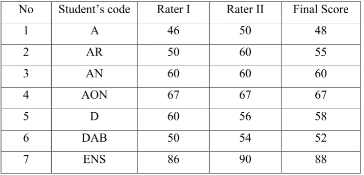
Table 4.1.1. Score of test of the students in office administration program No Student’s code Rater I Rater II Final Score
1 A 46 50 48
2 AR 50 60 55
3 AN 60 60 60
4 AON 67 67 67
5 D 60 56 58
6 DAB 50 54 52
8 HMY 70 70 70
9 H 80 70 75
10 IA 86.6 86.6 87
11 II 70 60 65
12 IN 50 56.6 53
13 KH 60 63.2 62
14 KMB 80 86.6 83
15 MM 60 63.3 62
16 MFRH 70 73.2 72
17 PL 60 53.3 57
18 RAR 70 66.6 68
19 RW 60 66.6 63
20 SY 70 70 70
21 WR 50 53.3 52
22 YW 60 63.2 62
Based on the data above, it can be seen that the student’s highest score was 90 and the student’s lowest score was 50. The writer determined the range of score, class interval, and interval of temporary. They can be concluded using formula as follows:
The highest score (H) = 88
The lowest score (L) = 48
The range of score (R) = 𝐻 − 𝐿 + 1
= 88 − 48 + 1
Class interval (K) = 1 + (3.3) × 𝐿𝑜𝑔 𝑛
= 1 + (3.3) × 𝐿𝑜𝑔 22
= 1 + (3.3) × 1.342422
= 1 + 4.423
= 5.423
Interval of temporary = 𝑅𝐾= 415
= 8.2
The range of score was 41, class interval was 5, and interval of temporary was 8. It was presented using frequency of distribution in the following table:
Table 4.1.2. Frequency of distribution
Class (K)
Interval (I)
Freq. (F)
Mid-point (X)
Limitation of each
group
Freq. Relative
(%)
Freq. Cumulative
(%)
1 80-88 3 84 79.5-88.5 13.63 100
2 72-79 2 75.5 71.5-79,5 9.09 86.35
3 64-71 5 67.5 63.5-71,5 22.72 77.26
4 56-63 7 59.5 55.5-63,5 31.81 54.54
5 48-55 5 51.5 43.5-55,5 22.72 22.72
Total ∑ 𝐹=
22
∑ 𝐹𝑥=
100
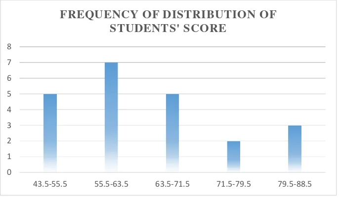
Figure 4.1. Frequency of Distribution of Students’ Score
The writer shown on the chart above the score of students in office administration program. There were five students who got score 43.5 to 55.5. Seven students who got 55.5 to 63.5. Five students who got 63.5 to 71.5. Two students who got the score 71.5 to 79.5. There were three students who got 79.5 to 88.5.
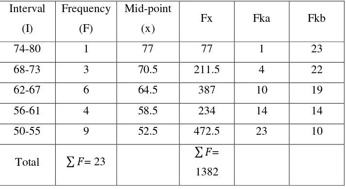
The next step, the writer tabulated the scores into the table for the calculation of mean, median, and modus as follows:
Table 4.1.3. The calculation of mean, median, and modus
Interval (I)
Frequency (F)
Mid-point
(x)
Fx Fka Fkb
80-88 3 84 249 3 22
72-79 2 75.5 151 5 19
64-71 5 67.5 337.5 10 17
56-63 7 59.5 416.5 17 12
0 1 2 3 4 5 6 7 8
43.5-55.5 55.5-63.5 63.5-71.5 71.5-79.5 79.5-88.5
48-55 5 51.5 257.5 22 5 Total ∑ 𝐹𝑥 = 22 ∑ 𝐹𝑥 =1311.5
a. Mean
Mx = ∑ 𝑓𝑥𝑁
= 1311,522
= 59.61
b. Median
Mdn = 𝑙 +12𝑁−𝑓𝑘𝑏
𝑓𝑖 × 𝑖
= 55.5 +1222−5
7 × 10
= 55.5 +1222−5
7 × 10
= 55.5 + 8.5
= 64
c. Modus
Mo = u + (fa+fb𝑓𝑎 )
= 55.5 + ((7−5)+(7−5)7−5 )
= 55.5 + (24)
= 55.5 + 0.5
= 56
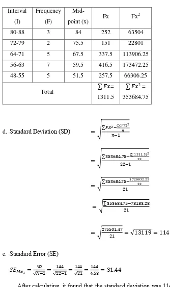
Table 4.1.4. The calculation of standard deviation
Interval (I)
Frequency (F)
Mid-point (x) Fx Fx
2
80-88 3 84 252 63504
72-79 2 75.5 151 22801
64-71 5 67.5 337.5 113906.25
56-63 7 59.5 416.5 173472.25
48-55 5 51.5 257.5 66306.25
Total ∑ 𝐹𝑥=
1311.5
∑ 𝐹𝑥2 =
353684.75
d. Standard Deviation (SD) = √∑ 𝐹𝑥
2−(∑ 𝐹𝑥)2 𝑛
𝑛−1
= √∑ 353684.75−(∑ 1311.5)222
22−1
= √∑ 353684.75−1720032.2522
21
= √∑ 353684.75−78183.2821
= √275501.4721 = √13119 = 114
e. Standard Error (SE)
𝑆𝐸𝑀𝑥1 =
𝑆𝐷 √𝑁−1=
144 √22−1=
144 √21 =
144
4.58= 31.44
2. The score of the students in marketing program
The data presentation of the sore of students in marketing program shown in the table frequency of distribution, the chart of frequency of distribution, the measurement of central tendency (mean, median, and modus) and the measurement of deviation standard. The score of the students in marketing program can be seen by following table:
Table 4.2.1. Score of test of the students in Marketing Program
No Student’s code Rater I Rater II Final Score
1 AS 60 66.6 63
2 DTF 56.6 56.6 57
3 EDAL 56.6 56.6 57
4 ET 63.2 63.2 63
5 HF 50 60 55
6 IW 50 53.3 52
7 IA 66,6 63.2 65
8 LNS 50 50 50
9 LAL 60 60 60
10 LDU 63.2 63.2 63
11 MA 66.6 70 68
12 MY 60 53.3 57
13 MRA 66.6 73.3 70
14 PA 56.6 53.3 55
15 PY 66.6 70 68
16 RD 80 80 80
18 RP 53,2 53.2 53
19 RA 66.6 63.3 65
20 ROM 66.6 63.3 65
21 SRD 50 60 55
22 ST 50 50 50
23 YP 50 53.3 52
Based on the data above, it can be seen that the student’s highest score was 90 and the student’s lowest score was 50. The writer determined the range of score, class interval, and interval of temporary. They can be concluded using formula as follows:
The highest score (H) = 80
The lowest score (L) = 50
The range of score (R) = 𝐻 − 𝐿 + 1
= 80 − 50 + 1
= 31
Class interval (K) = 1 + (3.3) × 𝐿𝑜𝑔 𝑛
= 1 + (3.3) × 𝐿𝑜𝑔 23
= 1 + (3.3) × 1.361727
= 1 + 4.493701
Interval of temporary = 𝑅𝐾= 315
= 6.2
The range of score was 31, class interval was 5, and interval of temporary was 6. It was presented using frequency of distribution in the following table:
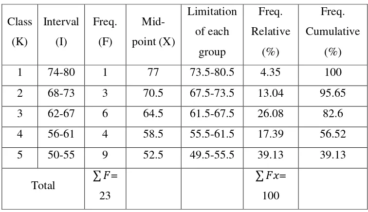
Table 4.2.2. Frequency of distribution
Class (K)
Interval (I)
Freq. (F)
Mid-point (X)
Limitation of each
group
Freq. Relative
(%)
Freq. Cumulative
(%)
1 74-80 1 77 73.5-80.5 4.35 100
2 68-73 3 70.5 67.5-73.5 13.04 95.65
3 62-67 6 64.5 61.5-67.5 26.08 82.6
4 56-61 4 58.5 55.5-61.5 17.39 56.52
5 50-55 9 52.5 49.5-55.5 39.13 39.13
Total ∑ 𝐹= 23
∑ 𝐹𝑥=
100
Figure 4.2. Frequency of Distribution of Students’ Score
It can be seen from the chart above the score of students in office administration program. There were nine students who got score between 49.5 to 55.5. Four students who got 55.5 to 61.5. Six students who got 61.5 to 67.5. Three students who got the score 67.5 to 73.5. There a student who got 73.5 to 80.5.
The next step, the writer tabulated the scores into the table for the calculation of mean, median, and modus as follows:
Table 4.2.3. The calculation of mean, median, and modus
Interval (I)
Frequency (F)
Mid-point
(x) Fx Fka Fkb
74-80 1 77 77 1 23
68-73 3 70.5 211.5 4 22
62-67 6 64.5 387 10 19
56-61 4 58.5 234 14 14
50-55 9 52.5 472.5 23 10
Total ∑ 𝐹= 23 ∑ 𝐹=
1382
0 2 4 6 8 10
49.5-55.5 55.5-61.5 61.5-67.5 67.5-73.5 73.5-80.5
a. Mean
Mx = ∑ 𝑓𝑥𝑁
= 138223
= 60.08
b. Median
Mdn = 𝑢 +12𝑁−𝑓𝑘𝑎
𝑓𝑖 × 𝑖
= 55.5 +1223−13
10 × 6
= 55.5 +−1.510 × 6
= 55.5 − 0.9 = 54.6
c. Modus
Mo = u + (fa+fb𝑓𝑎 )
= 55.5 + (5+105 )
= 55.5 + (155)
= 55.5 + 0,3
= 55.8
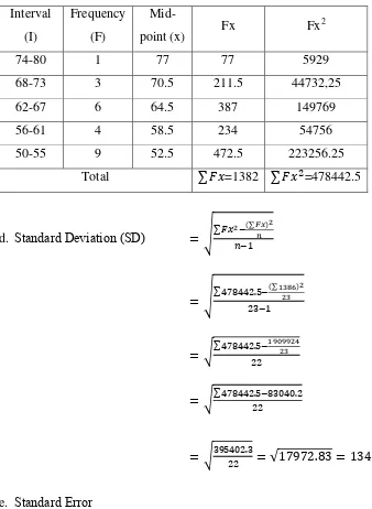
Table 4.2.4. The calculation of standard deviation
Interval (I)
Frequency (F)
Mid-point (x) Fx Fx
2
74-80 1 77 77 5929
68-73 3 70.5 211.5 44732,25
62-67 6 64.5 387 149769
56-61 4 58.5 234 54756
50-55 9 52.5 472.5 223256.25
Total ∑ 𝐹𝑥=1382 ∑ 𝐹𝑥2=478442.5
d. Standard Deviation (SD) = √∑ 𝐹𝑥
2−(∑ 𝐹𝑥)2 𝑛
𝑛−1
= √∑ 478442.5−(∑ 1386)223
23−1
= √∑ 478442.5−190992423
22
= √∑ 478442.5−83040.222
= √395402.322 = √17972.83 = 134
e. Standard Error
𝑆𝐸𝑀𝑥2 =
𝑆𝐷 √𝑁−1=
134 √23−1=
134 √22 =
134
4.69= 28.57
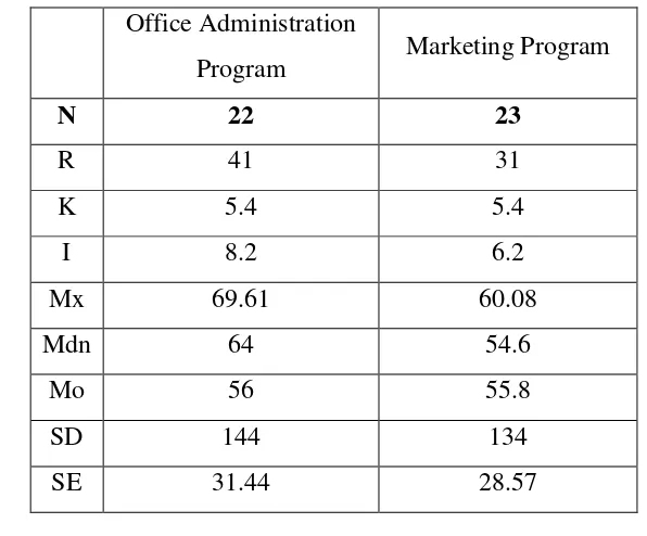
3. The Result of Data Analysis
Based on the analysis above, the writer concluded the result in following the table:
Table. 4.3. The data of test score of the students in office administration and marketing programs
Office Administration
Program Marketing Program
N 22 23
R 41 31
K 5.4 5.4
I 8.2 6.2
Mx 69.61 60.08
Mdn 64 54.6
Mo 56 55.8
SD 144 134
SE 31.44 28.57
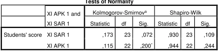
4. Testing of Normality and Homogeneity a. Normality test
Table 4.4.1. Normality Test of students of office administration and marketing programs
Tests of Normality
XI APK 1 and
XI SAR 1
Kolmogorov-Smirnova Shapiro-Wilk
Statistic df Sig. Statistic df Sig.
Students' score XI SAR 1 ,173 23 ,072 ,930 23 ,109
XI APK 1 ,115 22 ,200* ,944 22 ,244
The table showed the result of normality test using SPSS 22 program. To know the normality of data, the formula could be seen as follows:
If the number of sample. > 50 = Kolmogorov-Smirnov If the number of sample. < 50 = Shapiro-Wilk
Based on the number of data the writer was 45 < 50, so to analyzed normality data was used Shapiro-Wilk. The next step, the writer analyzed normality of data used formula as follows:
If Significance > 0.05 = data is normal distribution If Significance < 0.05 = data is not normal distribution
Based on data above, significant data of students of office administration and marketing programs used Shapiro-Wilk was 0.109 > 0.05 and 0.244 > 0.05. It could be concluded that the data was normal distribution.
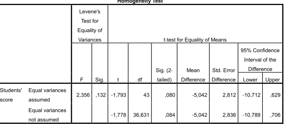
b. Homogeneity test
Table 4.4.2. Homogeneity test of students of office administration and marketing programs
Homogeneity Test
Levene's Test for Equality of
Variances t-test for Equality of Means
F Sig. t df
Sig. (2 -tailed)
Mean Difference
Std. Error Difference
95% Confidence Interval of the
Difference Lower Upper Students'
score
Equal variances
assumed 2,356 ,132 -1,793 43 ,080 -5,042 2,812 -10,712 ,629
Equal variances
not assumed -1,778 36,631 ,084 -5,042 2,836 -10,789 ,706
The table showed the result of Homogeneity test calculation using SPSS 21.0 program. To know the Homogeneity of data, the formula could be seen as follows:
If Sig. > 0,01 = Equal variances assumed or Homogeny distribution
If Sig. < 0,01 = Equal variances not assumed or not Homogeny distribution
5. Testing Hypothesis
In order to calculate the result of data analysis, the writer calculated it using t test. There were manual calculation and SPSS Program version 22.
a. Testing hypothesis using manual calculation
The computation for the independent t test. First, writer calculate Error Standard of differences mean as follows:
𝑆𝐸𝑀𝑥1 − 𝑆𝐸𝑀𝑥2 = √(𝑆𝐸𝑀𝑥1)2+ (𝑆𝐸𝑀𝑥2)2
𝑆𝐸𝑀𝑥1 − 𝑆𝐸𝑀𝑥2 = √(31.44)2+ (28.57)2
𝑆𝐸𝑀𝑥1 − 𝑆𝐸𝑀𝑥2 = √988.47 + 816.24 = √1804.71 = 42.48
The next step, the writer calculated testing hypothesis as follows:
𝑡 = 𝑋1−𝑋2
𝑆𝐸𝑀𝑥1−𝑆𝐸𝑀𝑥2
𝑡 =59.61−60.0842.48
𝑡 =−0.4742.48 = −0.011
degrees of freedom for the t test for independent means are 𝑛1+
𝑛2− 2.51
df = 𝑛1 + 𝑛2 − 2
= 22 + 23 − 2
= 43
The calculation above showed that degrees of freedom (df) was 43 at 5% level of significant = 2.018. It meant the observed ratio of -0.011 was smaller than 2.018. It could be interpreted that Ha stating that there is a significant difference on students’ ability of the students of Office Administration and Marketing Programs in writing application letter was rejected and Ho stating that there is no significant difference on students’ ability of the students of Office Administration and Marketing Programs in writing application letter was accepted. It meant that there is no significant difference on students’ ability of the students of Office Administration and Marketing Programs in writing application letter at the eleventh-grade students of SMKN 2 Palangka Raya.
b. Testing hypothesis using spss 22 program
Meanwhile, the calculation of ttest using SPSS 22 program can
be seen in the following table:
Table 4.5.1. Mean, Standard deviation, and standard error using SPSS 22 program.
Group Statistics
XI APK 1 and XI SAR 1 N Mean Std. Deviation Std. Error Mean
Students' score XI SAR 1 23 59,91 7,489 1,562
XI APK 1 22 64,95 11,103 2,367
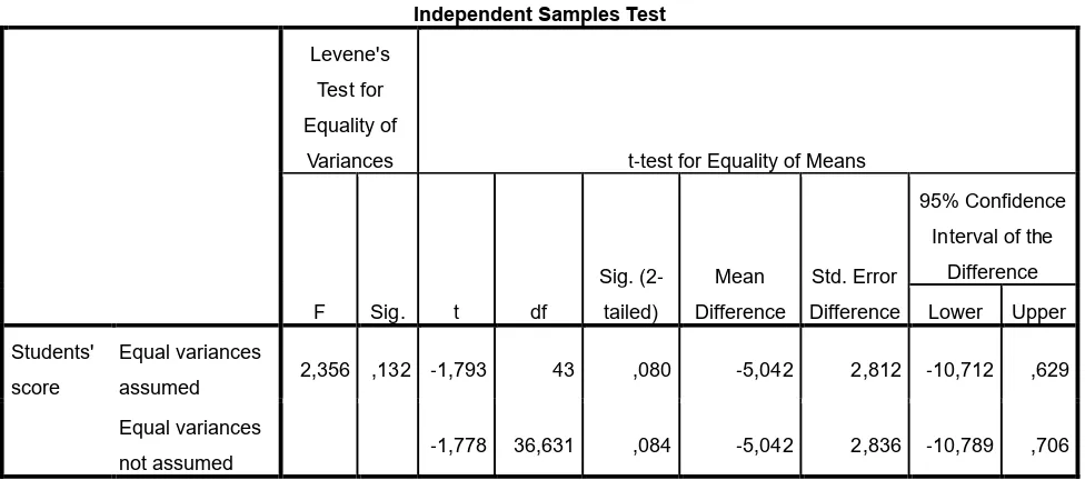
Table 4.5.2. Independent sample test using SPSS 22 program Independent Samples Test
Levene's Test for Equality of
Variances t-test for Equality of Means
F Sig. t df
Sig. (2 -tailed)
Mean Difference
Std. Error Difference
95% Confidence Interval of the
Difference Lower Upper Students'
score
Equal variances
assumed 2,356 ,132 -1,793 43 ,080 -5,042 2,812 -10,712 ,629
Equal variances
not assumed -1,778 36,631 ,084 -5,042 2,836 -10,789 ,706
letter at the eleventh-grade students of SMKN 2 Palangka Raya was accepted at 5% level of significance.
B. Discussion
The result of the analysis showed that there is no any significant difference on students’ ability between Office Administration Program (APK) And Marketing Program (SAR) in writing application letter at the eleventh Grade Students of SMKN 2 Palangka Raya. It could be proved from the students’ score that the score of students in office administration program was not significant difference with the score of students in marketing program. It was found the mean of students in office administration program (X1) was
59.61 and the mean of students in marketing program (X2) was 60.08.
Furthermore, the deviation standard of students in office administration program was 144 and the deviation standard of students in marketing program was 143. Then, those results were compared using t-test with pooled variant formula and it was found that tobserved was -0,011 and ttable was 2,018. It meant,
Ha was rejected and Ho was accepted based on the computation that found tobserved < ttable.
skills and create employment candidates who are competent, competitive, and independent in the secretarial field. Expertise in this program will educate students to be able to handle the administration of the company which includes handling incoming and outgoing mail, letters agenda, and schedule management. Meanwhile, Marketing Program is a program to equip students with the skills, knowledge and attitudes, and aims to equip students' abilities and skills in maximizing the potential with adequate facilities so as to produce skilled manpower in the field of marketing. Then, Improve the abilities and skills of students by involving schools and the World Business Council or World Industries to meet market needs.
Both explanation above shown the difference purpose between the students in office administration and marketing program. However, after the writer did research by giving the test to the students in different programs, in writing application letter in english subject, the result shown that there is no significant difference ability in writing application business letter between the students in office administration and marketing programs at the eleventh grade students of SMKN 2 Palangka Raya. It was supported by the theory that stated “English for specific purposes is a term that refers to teaching or
studying English for a particular career (like law, medicine) or for business in general.”52
52Veronika Burdová,., English for Specific Purposes (Tourist Management and Hotel
Based on the explanation above, the writer concluded some of possibilities could be caused why the students in the different of programs do not meant had different abilities in writing application business letter between the students in office administration and marketing programs at the eleventh grade students of SMKN 2 Palangka Raya. First, the students in different programs got the same chance materials on learning process. Second, the syllabus that being teachers’ reference in teaching English was the same syllabus. Third, the students in different programs got the same chance in time that five hours per weeks by description twice a week: two hours and three hours per meeting. The writer found all the factors by doing interview. The writer did the interview to the students and the teachers of office administration and marketing programs.