Chapter 14
Natural Resource Economics
14.1
The Intertemporal Nature of Natural
Resource Allocations
14.2
Present Values and Dynamic Efficiency
14.3
Nonrenewable Resource Extraction
A Simple Two-Period Hotelling Model14.4
Hotelling and Ricardian Scarcity Rents
14.5
Market Power in Nonrenewable Resource
Industries
14.6
Renewable Resources: The Fishery
Natural resources essential for human survival on planet earth include oxygen to breathe and water to drink. Our use of the natural environment is not, of course, limited to these most fundamental of resources. Within the atmospheric, terrestrial, and aquatic natural realms, we can identify scores of other natural resources whose exploitation or
conservation enhance the quality of human life. These resources include plant and animal species, the natural habitats that support those species, minerals, and energy hydrocarbons. As a factor of production, natural resources are often combined with labor and capital to produce a wide variety of final goods that consumers enjoy. Even a simple activity such as eating a tuna fish sandwich at a wood table in one’s natural gas-heated dining room, makes it easy to appreciate the contribution of natural resources to everyday life.
14.1
The Intertemporal Nature of Natural Resource Allocations
Natural resources come in two varieties: renewable and nonrenewable. Renewable resources, as the name implies, are those that potentially can be supplied to an economic system indefinitely. Many renewable resources are biological in nature; fish and trees are two prime examples. Their capability for growth and reproduction suggests the
possibility that they may be harvested on a sustainable basis. The mere potential for sustainability is just that. As we will discover, microeconomics has much to say about the circumstances that have taken some biological resources from the category of renewable (sustainable) to nonrenewable (extinct).
Nonrenewable resources are those with a finite stock, incapable of renewal in a length of time that is meaningful to us. Petroleum is nonrenewable, for our purposes, because millions of years are required for its natural formation. If it is all extracted and used up in the next few decades (which is quite unlikely), we say that it is exhausted. Not all nonrenewable resources are likely to be extracted until exhaustion. For many
nonrenewable resources, such as mineral ores, the marginal costs of extraction increase over time as it becomes increasingly difficult to physically raise the resource from the ever-deepening level of the mine to the surface of the earth. The quality of the ore may also deteriorate with the level of cumulative extraction. In the end, it may not be
economically viable to exhaust the resource; it may cost more to extract the last few units of the resource than anyone is willing to pay.
Regardless of whether a nonrenewable resource is extracted until exhaustion, current period extraction and use of the resource involves an intertemporal tradeoff. A unit of a nonrenewable resource used today is gone forever. It cannot be used to generate economic net benefits at some later date. The appropriate pattern of nonrenewable resource use over multiple time periods is thus a main focus of natural resource
harvested today can generate an immediate benefit to the consumer and thus immediate profit for the fisherman. What is the appropriate level of current period harvesting versus conservation for the future? To begin to answer these fundamental questions, we develop the dynamic analogue to the notion of economic efficiency presented in section 6.7 of Chapter Six. Once established, we can use the criterion of dynamic efficiency to evaluate the patterns of natural resource usage that we see under alternative institutional and property rights regimes.
14.2 Present Values and Dynamic Efficiency
In Figure 6-8, we considered the efficiency properties of a competitive market
equilibrium from an implicitly static (single period) perspective. That is, within a given time period, we argued that a competitive equilibrium maximizes the aggregate level of rents to consumers and producers. Where quantity demanded equals quantity supplied, there is an exhaustion of mutual benefits to buyers and sellers. Another way of
describing the efficiency property of the competitive equilibrium is to note that the
difference between consumers’ total willingness-to-pay (as measured by the area under the demand curve) and producers’ total cost (as measured by the area under the supply curve) is maximized at the point where quantity demanded equals quantity supplied. The difference between consumers’ total willingness-to-pay and producers’ total cost of production of a particular quantity is customarily referred to as the level of total net benefit generated by the equilibrium. Static efficiency requires the maximization of total net benefits in a given time period.
In the case of natural resource utilization, with its inherent intertemporal
tradeoffs, we must often compare the net benefits generated in one time period with those generated in another. Since income produced or received in different time periods have different present values, we cannot simply compare these amounts without correctly evaluating one amount in terms of the other. Recall from Chapter 10, that whether due to an explicit positive rate of time preference or simply a desire to smooth consumption over time in a growing production economy, capital markets establish a positive price for the earlier availability of the right to use goods. In monetary terms, interest is the premium for earlier availability of funds. In an economy with a positive rate of interest, a net benefit of $100 enjoyed a year from now is not worth as much as a $100 net benefit received today.
The present value criterion allows us to extend the notion of economic efficiency to a multi-period analysis. In a world of intertemporal tradeoffs, we say that an allocation of resources is dynamically efficient if it maximizes the sum of the present value of net benefits that can feasibly be generated over time. In considering an allocation of natural resource usage over time, we wish to compute the net benefits generated in each time period by the allocation, convert them to present values, and then add them up. A
14.3 Nonrenewable Resource Extraction
The simplest sort of model that allows for the passage of time is a two-period model.1 We will assume that a finite stock of a nonrenewable resource will be extracted over the course of two periods: period 1, representing the current period, and period 2 representing the future. Net benefits in both time periods are in inflation-adjusted dollars, and for ease of calculation, we will convert any net benefits generated in period 2 into a present value by assuming a real interest or discount rate of r = 0.50 = 50%. For simplicity, we will assume that an extracted unit of resource can be immediately consumed without any further need of processing. Demand in each period is given by Pt =11−Qt, where Pt is the per-unit price and Qt is the quantity of extraction and consumption in period t, with
t=1, 2. Assuming that the initial stock of the nonrenewable resource is 10 units, and that each unit of the resource may be extracted at a constant marginal cost of $1, what pattern of resource extraction would be dynamically efficient?
Table 14-1 provides for the calculation of total net benefits in each period as a function of the quantity extracted and consumed. Total willingness-to-pay is described by the area under the demand curve up to the quantity in question. With a linear demand curve, this area is easily computed as the sum of the area of a triangle and rectangle, and it is provided in column 3. Total cost is the product of the quantity extracted and the constant marginal extraction cost of $1. Total net benefit is provided in column 6, and it is simply the difference between total willingness-to-pay and total extraction cost. Marginal net benefit is given in column 7, and it is defined as the difference between marginal willingness-to-pay (price) and marginal extraction cost.
Table 14-1 Net Benefits from Extraction in a Particular Time Period
(1)A similar two-period model of resource extraction with constant marginal extraction cost is described at length in Tom Tietenberg’s upper-division text entitled,
If the nonrenewable resource were abundant (if the initial stock size was nearly infinite rather than 10), economic efficiency would dictate that we extract 10 units each period, for a sum total of 20 units over the course of two periods. At a quantity of 10 units extraction per period, price would equal marginal cost, and total net benefits in each period would be maximized. Maximizing the total net benefits in each period would, trivially, also maximize the present value sum of total net benefits over the two periods, and dynamic efficiency would be achieved. Without binding resource scarcity, the resource allocation problem would no longer involve intertemporal tradeoffs. However, in this example, with an initial endowment of only 10 units of the nonrenewable resource, we face the fundamental intertemporal tradeoff at the heart of exhaustible resource
economics. An additional unit of extraction in period 1 is necessarily at the expense of net benefits that could be generated by extracting the unit in period 2. With an initial stock size less than 20, we are confronted with precisely the exhaustible resource scarcity described and analyzed by the very influential economist Harold Hotelling in 1931.2
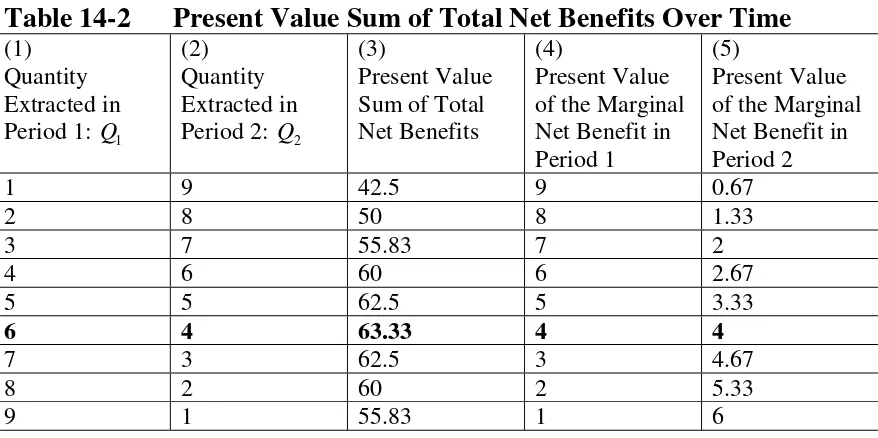
With an initial stock size of 10, Table 14-2 describes the feasible patterns of extraction over the two time periods. For instance, if we only extract 1 unit in period 1, then 9 units may be extracted in period 2. If 2 units are extracted in period 1, then 8 may be extracted in period 2, and so forth. For each of the rows in Table 14-2, Q1 andQ2 sum to 10, the size of our assumed nonrenewable resource endowment. Column 3 of the table describes the present value sum of the total net benefits generated by the various patterns of extraction. Extracting 6 units of the resource in period 1 and 4 units of the resource in period 2 achieves dynamic efficiency. Extracting 6 units generates total net benefits of $42 in period 1. Extracting 4 units generates total net benefits of $32 in period 2. In present value terms, these second period benefits equal $21.33 (=$32/(1+r) = $32/1.5). In the dynamically efficient solution to the resource allocation problem presented here, a present value sum of $63.33 of total net benefits is generated. The key to understanding the dynamic efficiency of this allocation is to focus on the present value of the marginal unit extracted in each period.
2
Table 14-2 Present Value Sum of Total Net Benefits Over Time
Notice from Table 14-2, that the sixth unit extracted in period 1 results in a marginal net benefit of $4. In period 2, the fourth extracted unit results in a marginal net benefit of $6, and that has a present discounted value equal of $4 (=$6/1.5) as well. In other words, in a world with constant marginal extraction costs and a scarce
nonrenewable resource, dynamic efficiency requires that the present value of marginal net benefits of extraction be the same across time periods. The last unit extracted in any time period must contribute the same to the present value bottom line. Otherwise, shifting extraction from periods with low present value marginal net benefits to those with high present value marginal net benefits would increase the present value sum of total net benefits. In the context of unchanging demand and constant marginal extraction cost, dynamic efficiency requires that the gap between price and marginal extraction cost rises at the rate of interest over time. In our example, it rises from $4 to $6. In a model with binding resource scarcity and a positive discount rate, extraction falls over time and price rises. The higher the discount rate, the more extraction will be shifted to the present because the future is relatively less valued. In our numerical example, only with a
discount rate of zero (r = 0) and an initial resource stock of 10 units would dynamic efficiency require 5 units be extracted in each period, because the net benefits generated in each period would be equally valued. If the discount rate is positive and the initial resource stock is not large enough to equate price and marginal extraction cost in all time periods, price will exceed marginal extraction cost. The difference between price and marginal extraction cost has many names in the nonrenewable resource literature. We have already described it as the marginal net benefit of extraction, but it is also called
marginal scarcity rent, royalty, marginal user cost, and, in a competitive industry,
marginal profit.
extraction over time. In every time period, price will exceed marginal extraction cost. With price greater than marginal cost, one might well ask, “why would the owner of a mining firm ever conserve the resource for later time periods? Why not expand current period extraction, and invest the profits at the prevailing rate of interest?” The answer must be that the mine owner expects price to rise over time, reflecting the increase in resource scarcity as exhaustible resource reserves decline. The individual mine owner correctly surmises that if everyone else in the industry exhausts their stock of the resource today, then they will be able to make windfall profits in the future as the sole remaining supplier. Of course, if every mine owner comes to this realization, then all will have the incentive to conserve some of their resource stock for the future. If the difference between price and marginal extraction cost is expected to rise at the rate of interest, then conservation of the resource for later time periods can be thought of as a rational capital investment. Hotelling argued that, in equilibrium, firm managers will be indifferent as to when they extract a marginal unit of the resource, because the present value of profit from marginal extraction will be the same in all periods.
14.4 Hotelling and Ricardian Scarcity Rents
In the model of extraction presented in the previous section, the resource was completely exhausted over time. The finite resource stock was characterized by constant marginal extraction costs, and the stock was not large enough to equate price and marginal cost in each time period. Consequently, dynamic efficiency required a gap between price and marginal extraction cost, a gap that rose at the rate of interest over time. In a world with eventual complete exhaustion of the resource, such a gap is referred to as a Hotelling scarcity rent. In keeping with the discussion of Chapter 6, recall that, ultimately, all rents arise from the inability to completely replicate resources. In the present instance, the nonrenewable resource stock, essential for production of certain final goods, is not replicable; rather, it is finite. For owners of finite resource stocks that will eventually be depleted, additional extraction of the resource in one time period is at the expense of profits that could have been generated in other time periods. The Hotelling scarcity rent (the difference between price and marginal extraction cost) represents the payment necessary to bring forth production of the marginal unit in the current rather than other time periods. This form of scarcity rent requires the economic viability of all units constituting the initial resource stock; it must be profitable to extract every last unit of the nonrenewable resource over time.
which there are intertemporal net benefit tradeoffs associated with the decision to extract more of the resource in a particular time period.
As previously discussed, for many nonrenewable resources, costs rise over time with cumulative extraction, so that not all units of the resource stock are worth extracting. However, even without complete exhaustion, scarcity rents may nonetheless arise, albeit, in a different form. In a world in which marginal extraction costs increase with the amount of cumulative extraction, a Ricardian scarcity rent will arise which reflects the additional costs imposed in future time periods from current period extraction. In this world, reserves of the resource are not of equal quality. Some units are more highly valued than others because they can be extracted at lower cost. When resource stock reserves are not of equal quality, the first units extracted will be those that are most profitable--those that can be extracted at relatively low cost. This phenomenon bares a striking similarity to the idea that the farmlands that will be cultivated first are those that are most fertile, and that the most productive farmlands will therefore earn a Ricardian rent.
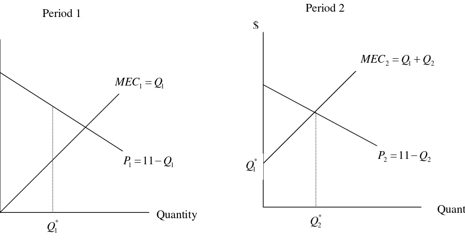
To illustrate the concept of Ricardian scarcity rent in the case of nonrenewable resources, reconsider the model of the previous section. In that model, every single unit of the resource stock could be extracted at a marginal cost of $1. Given the level of demand in each period, economic efficiency dictated complete exhaustion because extraction of all 10 units of the resource stock was profitable. What if, instead, only the first unit of the resource stock could be extracted for $1? What if the second unit could only be extracted for $2, the third for $3, and so forth? More precisely, in period 1, assume marginal extraction costs are MEC1=Q1. Entering period 2, Q1 units of the resource will have already been extracted, so marginal extraction costs in period 2 will be
MEC2 =Q1+Q2. If, for example, 4 units of the resource were extracted in period 1, then the first unit produced in period 2 (the fifth unit overall) would cost $5, and the second unit produced in period 2 (the sixth unit overall) would cost $6. If, on the other hand, 5 units of the resource were extracted in period 1, then the first unit produced in period 2 would cost $6, and the second would cost $7. In this formulation, the costs of extraction in period 2 now critically depend on the amount extracted in period 1. An additional unit extracted in period 1 increases the cost of every unit eventually produced in period 2 by $1 (relative to what second period costs would have been if an additional unit were not extracted in period 1).
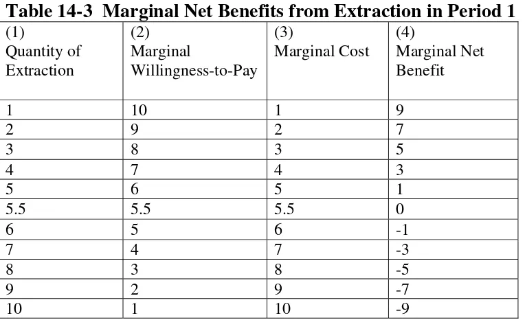
Table 14-3 Marginal Net Benefits from Extraction in Period 1
Clearly, extraction of six or more units in period 1 is not economically efficient because the marginal net benefits are negative at those levels. We never want to extract a unit of the resource if it costs more than some consumer is willing to pay. If we did not care about the level of second period net benefits, then we would extract 5.5 units in period 1 because marginal net benefits are zero at that level (price and marginal
extraction costs are both $5.50). First period total net benefits are maximized at Q1=5.5, meaning that the difference between total-willingness-to-pay and total extraction cost is at its greatest when Q1=5.5. However, because we do care about the net benefits generated in the second as well as first period, the dynamically efficient level of
extraction in period 1 will be less than 5.5. We want to extract less than 5.5 units in order to reduce the costs of second period extraction, even recognizing that extracting less than 5.5 units of the resource in period 1 entails a reduction in first period total net benefits. The achievement of dynamic efficiency requires that we sacrifice some first period net benefits in order to lower costs and increase net benefits in the second period. How much of a first period sacrifice should we be willing to make?
We should be willing to sacrifice precisely that amount of net benefit in period 1 that covers the present value increase in costs in period 2 from marginal extraction in period 1. In present value terms, we should be indifferent between extracting and
conserving a marginal unit of the resource in period 1. If we extract an additional unit in period 1, we generate some additional net benefits in that period. If we conserve an additional unit of the resource in period 1 (by not extracting it), we increase net benefits by reducing costs in period 2. Demand in period one is given by P1=11−Q1 and
extraction in period 1 creates a net benefit in that period equal to the subsequent present value increase in second period costs.
In our example, marginal costs increase with cumulative extraction, and dynamic efficiency requires Q1*=4.4 and Q2*=3.3. This pattern of extraction over the two periods maximizes the present value sum of total net benefits.3 The optimality of this solution is provided by the link between the marginal net benefit of first period extraction and its effect on costs in period 2. With Q1* =4.4 , P1=11−4.4=$6.6, and MEC1=$4.4. The marginal net benefit of extraction in period 1 is P1−MEC1=$2.2. With Q2* =3.3,
P2 =11−3.3=$7.7, and MEC2=Q1+Q2=$7.7. The marginal net benefit of extraction in period 2 is P2−MEC2=$0.0. The marginal net benefit is zero in period 2 because, by definition, in a two-period model, there is no period 3 that would provide benefits to consumers and producers.4 The gap between price and marginal extraction cost in period 1 is called a Ricardian scarcity rent at the margin, and it reflects the intertemporal
tradeoff between current and future extraction. It represents the net benefits in period 1 necessary to justify the increase in extraction costs and subsequent reduction in net benefits in the second period.
In our numerical example, marginal extraction costs in period 2 are described by MEC2 =Q1+Q2. Second period costs are a function of first period cumulative
extraction. The last unit extracted in period 1 increases the cost of producing all 3.3 units extracted in period 2 by $1 (relative to what second period costs would have been had the marginal unit not been extracted in period 1), for a total cost increase of $3.3. This cost increase in period 2 has a present discounted value of $2.2 (= $3.3/(1+r) = $3.3/1.5), which is, of course, precisely the value of the marginal net benefit of extraction in period 1. The marginal scarcity rent in period 1 is this $2.2. Even though price exceeds
marginal cost by $2.2, production of more than 4.4 units of the resource in period 1 would be dynamically inefficient because it would entail too large an increase in extraction costs in the next period. The dynamically efficient pattern of extraction is presented graphically in Figure 14-1.
3
For those with a background in calculus, these results are formally derived in an appendix at the end of this chapter.
4
Every additional unit of the resource extracted in period 1 shifts the marginal extraction cost curve in period 2 vertically by a unit. The positive gap between price and marginal cost (the Ricardian marginal scarcity rent) that is present in period 1 disappears in period 2. In the final period, price equals marginal cost, and there are no scarcity rents. This result generalizes to models with more than two time periods.5 The increasing marginal costs of extraction in our numerical example are sufficient to preclude exhaustion of the resource stock. By the end of the final time period, a total of Q1*+Q2*=4.4+3.3=7.7 units of the resource are extracted, and 2.3 units of the nonrenewable resource are left behind in the ground. Producing Q2*=3.3 units in period 2, the final time period, is efficient because the willingness-to-pay for marginal extraction (price) by some consumer is just sufficient to just cover the cost of marginal extraction. Production greater than Q2*=3.3 units in period 2 would be inefficient because marginal extraction cost would exceed marginal-willingness-to-pay.
5
The distinction between Hotelling and Ricardian scarcity rents is discussed at length by Levhari and Liviatan in their paper “Notes on Hotelling’s Economics of Exhaustible Resources,” Canadian Journal of Economics, 10: 1714-192, 1977.
Q1*
$
MEC1=Q1
P1=11−Q1
Quantity Period 1
Q2*
$
Period 2
MEC2 =Q1+Q2
P2=11−Q2
Quantity
Figure 14-1 Dynamic Efficiency in a Model with Increasing MEC
When marginal costs rise sufficiently with cumulative extraction, so that the resource stock is not exhausted, Ricardian scarcity rents decline to zero in the last period. Unlike the Hotelling scarcity rents that emerged in our previous model with constant marginal extraction costs and complete exhaustion of the resource stock, Ricardian scarcity rents do not rise at the rate of interest over time. In a model with increasing marginal extraction costs and incomplete exhaustion, Ricardian scarcity rents actually decline over time! In period 1, the Ricardian scarcity rent at the margin is
P1−MEC1=$2.2, and in the final time period it is P2−MEC2 =$0.0. The popular characterization that nonrenewable resource economics establishes the proposition that scarcity rents rise at the rate of interest is incorrect when it comes to the case of resources that will not be completely exhausted.
14.5 Market Power in Nonrenewable Resource Industries
Due to the presence of Hotelling and/or Ricardian scarcity rents, price will often exceed the marginal cost of production in nonrenewable industries even if they are perfectly competitive. This feature distinguishes nonrenewable resource industries from most others because a perfectly competitive market structure usually results in an equating of price and marginal cost. Moreover, in nonrenewable resource industries, price will often exceed marginal cost for a completely different reason as well. Many of these industries are not perfectly competitive. Several important mineral and fossil fuel markets have been affected by the actions of suppliers who have successfully, from time to time, organized cartels aimed at restricting output and raising price.
As discussed in Chapter 12, the simple formation of a cartel is no guarantee of its success. The biggest difficulty facing cartel members in their attempt to collectively restrict output and increase profits is the incentive each member has to cheat on the cartel agreement. If all other members of a cartel are abiding by an agreement and its inherent production quotas, price will be higher than it would otherwise be. This makes it very profitable, in the short run, for the cartel member in question (a firm or country that owns a nonrenewable resource stock) to expand output beyond the limits proscribed by the production quota. If detected, this form of cheating will often lead to a general
more heavily the cartel member discounts future period profits relative to current period profits, the more likely it is to cheat for short run gain.
In addition to the size of the discount rate, the magnitude of cartel profitability is another very important factor that influences an individual member’s incentive to cheat. How large are the cartel’s future profits (and the member’s share of them) that are put at risk by cheating? The answer to that question depends, in part, on the percentage of the nonrenewable resource stock controlled by members of the cartel. Not all producers of nonrenewable resources choose to belong to cartels even if they have been formed. In an industry that has been partially cartelized, nonmembers of the cartel are said to constitute a competitive fringe. When cartel members cooperate and voluntarily restrict their output, price rises initially (relative to what it would have been), inducing a positive response in the quantity supplied from the competitive fringe. The supply response of the competitive fringe therefore dampens the initial price rise and it lowers cartel members’ profits.
The size of the competitive fringe determines, to a large degree, the level of cartel profitability. The larger the competitive fringe, in terms of numbers of firms and the size of the resource stocks they own, the smaller the profitability of the cartel. If most of a resource stock is owned and controlled by a competitive fringe, the benefit to
cartelization is small because the cartel will not be able to substantially increase equilibrium price. If, on the other hand, the resource stock is completely owned and controlled by cartel members (i.e., if there is no competitive fringe), then the benefit to cartelization is potentially very large. In that case, the cartel could, through its collective production restrictions, theoretically mimic the behavior of a monopolist and generate monopoly-level profits for the group.
When the Organization of Petroleum Exporting Countries (OPEC) was formed, it controlled approximately two-thirds of the world’s estimated oil reserves. Similarly, the International Bauxite Association (IBA) had an overwhelming market share of the noncommunist world’s bauxite production by the mid-1970s. In the case of these two important nonrenewable resources, the cartels were large compared to the size of the competitive fringe. The potential benefit from cartelization (relative to behaving in a perfectly competitive fashion) to members in these two industries has been estimated to be quite substantial.6 OPEC has dramatically increased the price of oil periodically, and IBA tripled the price of bauxite for a while (although it has not been as successful recently). By way of contrast, the International Council of Copper Exporting Countries has never been able to substantially raise copper prices. It has been an unsuccessful cartel primarily because of its small market share. The competitive fringe in the copper industry accounts for the majority of the world’s production of that commodity.
Economic theory tells us that when the benefits to cartelization are small, it is hard to keep members from cheating on production quotas because they are not risking a particularly profitable future anyway.
Cartels are not the only avenue for the exercise of market power. Some firms and countries have been naturally endowed with vast reserves of nonrenewable resources. The International Nickel Company of Canada (Inco) is, far and away, the largest firm in
6
the international nickel industry, and for much of the twentieth century, it possessed a majority market share in sales of nickel in the noncommunist world market. Historically, Inco’s largest mining operations have been located in the Sudbury basin of Ontario, Canada. The basin was formed some 1.85 billion years ago when an asteroid 6 to 12 miles in diameter crashed into our planet, cracking the earth’s crust, and producing vast deposits of minerals containing nickel, copper, and several precious metals. Nickel is an important intermediate input to the production of many commodities because, among other things, it is used in the production of stainless steel. Inco is a vertically integrated firm, in that, it not only extracts nickel ore, but it also processes the ore into finished products like sheets of rolled nickel. Given its dominant position in the nickel market and the importance of nickel in a variety of applications, Inco has been the subject of several investigations by economists regarding scarcity rents, and most recently, the issue of its exercise of near-monopoly market power.
In an article published in 2002, Ellis and Halvorsen describe a methodology to explain the gap between price and marginal cost of production as the sum of resource scarcity rent and market power markup.7 Their methodology is applied to a dataset for Inco for the time period from 1947 to 1992. They estimate that the components of an average price of $2.75 received for a pound of finished nickel product are marginal costs of production (in terms of labor and capital costs) of $0.83, marginal scarcity rents of $0.22, and an average market power markup of nearly $1.70. In an earlier study of Inco, economist Robert Cairns argued that Inco’s nickel reserves are so abundant that there is no Hotelling scarcity rent because the reserves are unlikely to be exhausted, and
therefore, the only relevant source of a scarcity rent for nickel is the effect that current period extraction has on future costs.8 Indeed, Ellis and Halvorsen find evidence for a Ricardian scarcity rent because they find that current period and cumulative extraction does, in fact, increase future extraction costs. However, as an empirical matter, these Ricardian scarcity rents only partially explain the gap between price and marginal cost because they pale in comparison to the large market power markups that Inco seems to successfully establish given its huge market share.
14.6 Renewable Resources: The Fishery
In contrast to nonrenewable resources, renewable resources are those that can potentially be supplied to an economic system indefinitely. Many renewable resources are
biological in nature. Their capability for growth and reproduction suggests the possibility that they may be harvested on a sustainable basis. In this section, we consider the
exploitation of fish stocks by commercial harvesters. Most fish that are caught commercially are for direct human consumption, but fish are also used as an input to
7
Ellis and Halvorsen, “Estimation of Market Power in a Nonrenewable Resource Industry,” Journal of Political Economy, 110: 883-899, 2002. All dollar figures in the subsequent text are in constant (inflation-adjusted) 1983 U.S. dollars.
8
Cairns, “An Application of Depletion Theory to a Base Metal: Canadian Nickel,”
production of other commodities like animal feed and fertilizer. The world now harvests annually over 100 million metric tons of fish commercially, and fish are a very important source of protein for much of the world’s population. Despite the overall growth in fish harvests over time, many of the world’s fisheries are in trouble. Water pollution, loss of spawning habitat, and overfishing have all contributed to the decline of many important fish species. In this section of the chapter, we describe a simple model of biological growth for a single fishery and discuss the possibility of sustainable harvest. In subsequent sections, we describe the economic incentives that can lead to an overexploitation of fish stocks and possible regulatory remedies for overfishing.
A fishery generally consists of a biomass of fish, typically a single species that resides in a well-defined geographical area that might be caught by a particular fishing technique. We might, for instance, refer to the Northern Pacific Halibut Fishery or the drift gillnet salmon fishery of Prince William Sound. The biomass of a fishery is the conventional measure of stock size; it is essentially the aggregate weight of the fish stock in a particular geographical area. Fish, like other animal species, need food and a suitable habitat to thrive. The size of a fishery depends upon many environmental factors
including ocean currents and temperature, water qualities like oxygen content, food supplies, and the prevalence of predators. Holding these ecosystem characteristics
constant for the moment, let us consider the possibilities for the natural growth of the fish stock in a particular time period.
Net natural growth consists of the maturation of the existing stock, additions to the stock from reproduction, and reductions to the stock from natural mortality. The amount of net natural growth over the course of a time period will be largely influenced by the size of the fish stock at the beginning of the time period. At small biomass levels, the abundance of ecosystem resources may promote rapid rates of growth. At larger biomass levels, growth usually slows until the fish stock finally reaches it maximum feasible size for the ecosystem characteristics, the so-called carrying capacity of the habitat. The logistic model of population growth postulated by the biologist P.F. Verhulst in 1838 is a famous example of a growth function exhibiting these
characteristics. WithXt as the stock size of the fishery in period t, the one-period logistic growth function is F(Xt)=gXt(1−Xt k)=gXt−gXt
2
k. In this quadratic formulation, g is referred to as the intrinsic growth rate, and k is the carrying capacity stock size. Notice that when evaluated at stock levels of Xt =0 or Xt =k, the net natural growth is zero. In the absence of human harvesting activities, the logistic growth function predicts that a fish stock introduced to an ecosystem for the first time will eventually grow to its carrying capacity size.
The quantity of fish harvested in a particular period of time is directly
proportional to the level of human effort devoted to the activity (as measured by some sort of composite index of the number of fishing boats, the size of fishing crews, types of fishing gear, amount of time spent at sea, etc.) and the size of the fish stock. For
′
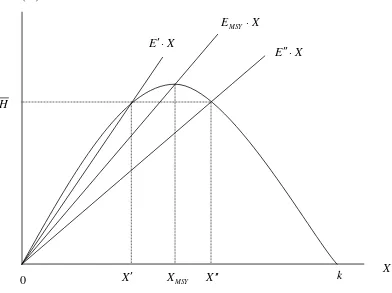
X XMSY X ′ ′
for a fixed level of effort, the quantity harvested increases as stock size increases. The slope of each harvest line is the effort level. In Figure 14-2, E ′ >EMSY > ′ ′ E .
Once we consider the possibility of human harvesting activity, we can determine whether the stock will grow or decline in size by noting that the change in stock size between period t and (t+1) is simply the difference between the amount of net natural growth and the quantity harvested in period t: Xt+1−Xt =F(Xt)−Ht. If F(Xt)>Ht, the stock will be larger at the beginning of period (t+1) than it was at the beginning of period t. Just the opposite will be true if Ht >F(Xt). When F(Xt)=Ht, the stock size remains unchanged between periods t and (t+1). In this special case, we say that the stock size is in a steady-state. The amount harvested equals the amount of biological growth, so the stock size remains constant. That is, in period (t+1), if F(Xt+1)=Ht+1, then, once again,
the stock size will be the same entering period (t+2) as it was in periods t and (t+1). With a constant stock size over multiple time periods, the ecosystem generates a constant amount of biological growth in each period that can, theoretically, be sustainably harvested.
k
H
′
E ⋅X
′ ′
E ⋅X EMSY⋅X
F(X)
X
0
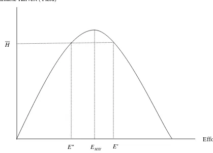
The situation in which F(Xt)=Ht =F(Xt+1)=Ht+1=F(Xt+2)=Ht+2, and so forth, is called one of sustainable harvest or sustainable yield. In Figure 14-2, the intersection of the three harvest lines with the growth curve represents three steady-state, sustainable yield scenarios. If the stock size is maintained at a level labeled as XMSY on the
horizontal axis, then the amount of one-period biological growth is maximized. That growth, measured in biomass terms, can be harvested on a sustainable basis, and it is called the maximum sustainable yield (MSY). If the stock is maintained at the level
XMSY, and the level of fishing effort is held constant at EMSY, then the harvest will be MSY=EMSY⋅XMSY =F(XMSY) every period. For many years, fisheries management authorities advocated a goal of harvesting fish stocks on a maximum sustainable yield basis. Of course, from the perspective of microeconomic theory, this criterion seems ad hoc. After all, we have thus far said nothing about the net benefits of fishing. We have not yet discussed the presumably diminishing marginal willingness-to-pay for fish harvests, nor have we discussed the costs of fishing as they relate to harvest or fish stock levels. Dynamic efficiency would dictate that we try to manage stock and harvest levels in such a way as to maximize the present value sum of economic net benefits that the fishery can generate over time, and a criterion of maximum sustainable yield is not necessarily consistent with that goal.
For any intermediate level of sustainable harvest (between zero and MSY), there are two distinct ways of producing that quantity of catch. In Figure 14-2, the
intermediate harvest level H can be sustained by employing a large amount of effort E ′ in combination with a relatively small stock level X ′ or by employing a relatively small amount of effort E ′ ′ while maintaining a large stock size X ′ ′ . That is,
H = ′ E ⋅ ′ X = ′ ′ E ⋅ ′ ′ X with E ′ > ′ ′ E and X ′ < ′ ′ X . We can think of the production of sustainable fish harvests as a function of two inputs with substitution possibilities: human fishing effort and fish stock. The costs of fishing in period t can then appropriately be modeled as C(Ht,Xt) where Ht is the amount of fish harvested and Xt is the stock size. Holding the stock size constant, costs go up when we increase harvest because we must increase human fishing effort. Holding harvest levels constant, costs go down when the stock size is increased because we can decrease human effort levels and still catch the same amount of fish.
Although a full-fledged derivation of the steady-state stock and harvest levels consistent with dynamic efficiency is beyond the scope of this text, we can at least discuss the intertemporal tradeoffs involved in considering the benefits of marginal harvest versus marginal conservation of the fish stock.9 The benefit to harvesting an extra ton of fish today is the difference between what consumers are willing to pay for it and the marginal cost of catching it. On the other hand, if the marginal ton of fish is not caught today, fishing costs next period will be incrementally smaller because costs are a decreasing function of stock size, and by conserving the marginal ton of fish, the stock size is larger than it would have otherwise been. Moreover, conserving the marginal ton of fish today may contribute to additional biological growth between the current and next
9
Derivations of the conditions for dynamic efficiency for many standard fishery models can be found in Colin Clark, Mathematical Bioeconomics: The Optimal Management of Renewable Resources, New York: Wiley-Interscience, 1990.
Figure 14-3 Yield-Effort Curve
Sustainable Harvest (Yield)
Effort
′ ′
E E ′
H
time period because biological growth is a function of stock size. That additional growth can eventually be harvested for a marginal net benefit (the difference between price and the marginal cost of harvest). The decision to harvest or conserve the marginal ton of fish today is therefore an intertemporal one. The benefits of current period conservation will not be enjoyed until a later date, and so the discount rate will, in part, define the dynamically efficient stock size and harvest level. For dynamic efficiency to be attained, the marginal benefit of current period harvest must be equal to the present value of the marginal benefit of conservation. As we will see in the next section, common property fisheries are rarely dynamically efficient because the exploiters of the resource have no incentive to consider the societal benefits of marginal conservation when racing to catch fish against their fishermen rivals.
Compared to the stock size associated with maximum sustainable yield, XMSY, what is the dynamically efficient stock size? The answer is theoretically ambiguous. It is an empirical question. The answer depends upon the relative magnitude of the stock effect on fishing costs and the discount rate effect on the opportunity cost of maintaining stock sizes. The larger the reduction in fishing costs when stock size is increased, the larger the stock size we would like to maintain in steady-state, all other things being equal. The discount rate plays an opposite role in determining the optimal stock size. Just as in the case of nonrenewable resources, the higher the discount rate, the higher the opportunity cost (in terms of forgone current period net benefits) of maintaining any given resource stock size for the purpose of generating future net benefits. Therefore, higher discount rates are associated with smaller optimal fish stock sizes. While it is theoretically impossible to say whether the dynamically efficient stock size is larger or smaller than the stock size associated with maximum sustainable yield, we can
unambiguously say that dynamic efficiency requires a larger maintained stock size than the one that emerges in equilibrium in the common property open-access fisheries discussed in the next section.
14.7 Open-Access Common Property Fisheries
Ocean fisheries have historically been open-access resources. Anyone who wanted to fish could do so; nobody was excluded from the fisheries. When nobody has private property rights with respect to a resource, so we say that the resource is common property. Without established private property rights to fish in the sea, anyone who catches fish can keep them without paying fees to an owner. How much fishing effort should we expect to see in equilibrium in an open-access common property fishery? Economist H. Scott Gordon provided a disturbing answer in 1954.10 Gordon reasoned that individual fishermen have an incentive to expend effort until profits are zero. As long as additional effort (boats, time spent fishing, capital equipment, etc.) generates additional profits, fishermen will pursue additional harvest of a resource they view as free.
10
To see his argument more clearly, assume the price of fish harvest is a constant
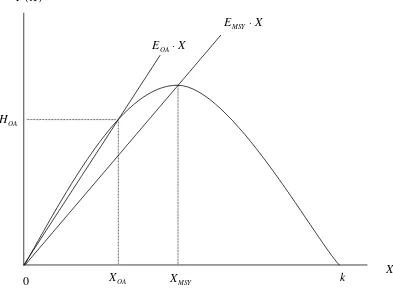
$p per unit. This assumption is made for graphical convenience and can be relaxed without affecting qualitative results. If we multiply the price of harvested fish by the quantity of fish that can be caught on a sustainable basis (as measured by the yield-effort curve of Figure 14-3), we obtain the total revenue (TR) curve presented below in Figure 14-4. It has the same shape as the yield-effort curve because we have simply multiplied that curve by a constant (price). Assume further that the marginal cost of effort is a constant $c per unit. The total cost of effort is then TC=c⋅E, and the total cost of effort can be graphed as a straight line with a slope of c.
The open-access equilibrium level of effort is EOA, and it is associated with the intersection of the total revenue curve and total cost line. Notice that the open-access level of effort is greater than the level associated with maximum sustainable yield:
EOA >EMSY. Profits to the fishermen are zero. All of the rents that could have accrued to the fishermen in this fishery have been dissipated, just as rents were dissipated in the common property farming example discussed in section 7.3 of Chapter 7. In our present fishery context, rents represent the net gains in the value of fish harvest over the cost of fishing effort employed to produce the harvest. There are no rents in an open-access
Figure 14-4 Open-Access Common Property Equilibrium
Total Revenue and Total Cost
Effort
TC=c⋅E TR
fishery because, in equilibrium, total revenue equals total cost. For levels of effort smaller than EOA, total revenue exceeds total cost, profits (rents) are positive, and
individual fishermen have the incentive to expend additional effort. In equilibrium, after new fishermen have entered the fishery and incumbent fishermen have expended
additional effort in the pursuit of profits, profits fall to zero; as a function of fishing effort, total revenue equals total cost, and average revenue equals average cost.
Figure 14-4 presents the open-access equilibrium in terms of fishing effort (the variable on the horizontal axis), but we can also describe the equilibrium in terms of harvest and fish stock. In equilibrium, total revenue equals total cost:
p⋅HOA =C(HOA,XOA) where HOAis the open-access level of industry harvest, XOA is the open-access level of fish stock, and C(HOA,XOA) is the total cost of fishing to the
industry. The equilibrium condition of zero profitability can also be expressed as
p=C(HOA,XOA) HOA. Price equals the average cost of harvest. As long as price exceeds the marginal cost of harvest, no fisherman has the incentive to conserve any fish (rather than harvest it immediately) because an individual fisherman has no property rights to the future benefits that current period conservation can bring, namely growth of the fish stock and lower fishing costs in the future. In an open-access common property fishery, if price is greater than the marginal cost of harvest, each fisherman realizes, “a fish not caught by me, will surely be caught by somebody else.” In the race to catch fish against their rivals, all suffer the fate of the tragedy of the commons: rents are completely dissipated.
What about the steady-state level of the fish stock in an open-access common property equilibrium? Is it larger or smaller than the level of fish stock associated with maximum sustainable yield (XMSY)? Recall, from Figure 14-2, that the slopes of harvest lines are equal to the effort level employed in catching fish. Since EOA >EMSY, the slope of the harvest line (function) associated with the open-access equilibrium is greater than that associated with maximum sustainable yield. The size of the fish stock in an open-access equilibrium is depicted in Figure 14-5. The open-open-access level of the fish stock,
XMSY EOA⋅X
HOA
XOA
H. Scott Gordon summarized the tragedy of the commons eloquently:
“There appears, then, to be some truth in the conservative dictum that
everybody’s property is nobody’s property. Wealth that is free for all is valued by none because he who is foolhardy enough to wait for its proper time of use will only find that it has been taken by another…the fish in the sea are valueless to the fisherman, because there is no assurance that they will be there for him tomorrow if they are left behind today. A factor of production that is valued at nothing in the business calculations of its users will yield nothing in income. Common property natural resources are free goods for the individual and scarce goods for society. Under unregulated private exploitation, they can yield no rent; that can be accomplished only by methods which make them private property or public (government) property, in either case subject to a unified directing power.”11
11
H. Scott Gordon, op. cit.
k EMSY⋅X
F(X)
X
0
As an example of open-access overfishing, consider the case of the Peruvian anchovy fishery of the 1960’s and 1970’s. It was one of the world’s most important fisheries, not because of any great demand for anchovies on pizza, but rather because anchovies were a primary ingredient in fishmeal and livestock feed. Its annual catch of over 10 million metric tons (10,000,000,000 kilograms) amounted to 15% of the total global catch of marine fisheries, including mammals and crustaceans.12 At its peak, the number of boats in Peru’s anchovy fleet is estimated to have been large enough to catch the entire annual U.S. harvest of yellowfin tuna and salmon in less than a week. The fleet was much larger than needed to catch even the maximum sustainable yield of the
Peruvian anchovy fishery. By the early 1970’s, the anchovy stock was severely depleted, and when El Niño arrived in 1973, the warming of the ocean, in combination with open-access fishing, led to the near collapse of the fishery and a dramatic increase in world food prices. Unfortunately, the case of the Peruvian anchovy fishery is not unique.
The cod, haddock, and yellowtail flounder fisheries of New England, the halibut fishery of the Northern Pacific, and the bluefin tuna fisheries of Australia and New Zealand (to name but a few) have all historically suffered the aforementioned symptoms of overharvesting and subsequent stock depletion typical of open-access common property regimes.13 All these fisheries are now regulated, several by a system of
individual transferable quotas (ITQ). ITQ regulatory systems introduce private property rights into fisheries that were previously common property.
Suppose regulatory authorities wish to allow 1,000 tons of fish to be caught each year in a particular fishery. A system of ITQ can be introduced in which 1,000 quotas are distributed to fishermen, each quota entitling the holder to catch 1 ton of fish annually. If a fisherman owns 5 quotas, he may legally catch 5 tons of fish anytime he desires during a particular year. If he wishes to catch an additional sixth ton of fish, he must purchase a quota from some other fisherman. A fisherman will purchase an additional quota in the marketplace if the present discounted value of the stream of profits it generates over time exceeds its price. The transferability of quotas ensures that the most efficient fishermen will continue to operate in the fishery in the long run because they value the property rights inherent in the quotas more highly than less efficient fishermen. Relatively efficient fishermen will be net buyers in the market for quotas; inefficient fishermen will be net sellers of quotas.
Before the introduction, in the 1990’s, of ITQ regulations for the Canadian and U.S. Pacific halibut fisheries, they were regulated as derby fisheries. In a derby fishery, the government sets a limit on the total allowable catch (TAC) for the year, and the fishery is then opened on a specific date. As soon as the TAC is reached, the fishery is closed for the year. The problem with this form of regulation is that the fish in the sea are still essentially common property. During the derby season, fishermen still have the incentive to race against one another in an attempt to capture profits from a resource they view as free. Derby fishing is very dangerous, as fishermen will often fish for 36 or more hours without sleep in order to increase their harvest and share of the TAC. In a derby
12
Colin Clark, op. cit. 13
fishery, the TAC is harvested in a very short amount of time (less than a week in the halibut fisheries before the introduction of ITQ). Fish markets are temporarily flooded with a year’s worth of halibut, depressing prices and revenues to fishermen. Consumers can only purchase fresh halibut for a brief time, and so they, too, suffer from the
incentives created by derby systems that have fishermen harvesting fish so quickly. Consumers are better off when the TAC is harvested over a longer fishing season. Under the new systems of ITQ regulations, the Canadian and U.S. halibut fisheries are enjoying much longer fishing seasons. Fresh halibut is now supplied to markets over many months instead of just a few days because fishermen do not need to race against each other. In their quota holdings, fishermen have a guaranteed property right to catch a specified quantity of fish anytime during the course of a year that they deem most profitable. In equilibrium, the harvested TAC is more evenly distributed over the year, and prices and profits have dramatically increased.
Appendix 14-1
Ricardian Rents in a Dynamically Efficient Model of Nonrenewable
Resource Extraction with Increasing Marginal Extraction Costs
In the two-period model presented in section 14.4, price in each period is given by
Pt =11−Qt, so total willingness-to pay, the area under the demand curve, is
2 , and total extraction cost in the second period is
2
synonymous with maximizing the present value sum of economic net benefits over the
two periods:
The two first-order necessary conditions for maximization are
Q1*=4.4 , P1*=11−4.4=$6.6, MEC1=$4.4, Q2*=3.3, P2*=11−3.3=$7.7, and
MEC2=4.4+3.3=$7.7. The marginal net benefit of extraction in period 1 (the
Ricardian rent in period 1) is MNB1=P1−MEC1=6.6−4.4=$2.2. The present value
increase in costs in period 2 from marginal extraction in period 1 is Q2 *
1.5= 3.3
1.5=$2.2
because the last unit extracted in period 1 increases the cost of extraction of every unit
produced in period 2 by $1. The Ricardian rent in period 2 is zero because price equals
marginal cost. Of the 10 units in the initial resource stock, 2.3 units
(=10−Q1*−Q2*=10−7.7) remain in the ground and are not extracted by the end of
CHAPTER SUMMARY
Renewable resources are those that can be supplied to an economic system indefinitely. Many resources are renewable because they are capable of biological growth. Nonrenewable resources are those with a finite stock, incapable of renewal in a length of time that is meaningful to us.
When current period use of a natural resource reduces the net benefits that can be generated in future time periods, we say that we are facing an intertemporal tradeoff. An allocation of resources is dynamically efficient if it maximizes the present value of net benefits that can be feasibly generated over time.
When a nonrenewable resource stock is exhausted over time in a context of constant marginal extraction costs, the gap between price and marginal extraction cost in a particular time period is called the marginal net benefit of extraction or the Hotelling scarcity rent. In a dynamically efficient extraction program, Hotelling scarcity rents will rise at the rate of interest. The present value of marginal net benefits of extraction will be the same in all time periods.
In a model of nonrenewable resource extraction without exhaustion, a Ricardian scarcity rent will arise. A Ricardian scarcity rent is the marginal net benefit of extraction necessary to justify the present value increase in extraction costs in all future time periods from marginal extraction in the current time period. Ricardian scarcity rents do not rise at the rate of interest.
Many nonrenewable resource markets are imperfectly competitive; consequently, in addition to the presence of scarcity rents, price often exceeds marginal cost because of the exercise of market power by resource cartels or dominant firms. The mere existence of cartels does not guarantee their success because members of cartels have a short run incentive to produce in excess of their production quotas.
When the quantity of fish harvested equals the amount of net natural growth, the fish stock is in steady-state and the fish harvest is described as a sustainable yield. Maximum sustainable yield is an ad hoc management criterion without economic merit. Intermediate levels of sustainable yield may be caught by either employing small levels of fishing effort in combination with large maintained stock sizes, or by employing large levels of fishing effort in combination with small maintained stock sizes.
conserve fish stock in a dynamically efficient way because they have no property rights to the future net benefits that appropriate conservation can supply.
Regulation by means of a system of individual transferable quotas (ITQ) is usually more efficient than by total allowable catch (TAC) alone. ITQ establish private property rights for individual fishermen, thereby eliminating the incentive to inefficiently race against other fishermen in harvesting fish.
REVIEW QUESTIONS
1. Why might perfectly competitive nonrenewable resource industries be dynamically efficient?
2. Why do cartels often fail in their effort to significantly raise the market price of nonrenewable resources? How does the size of the competitive fringe affect the cartel’s success?
3. Why are natural resource problems characterized by intertemporal tradeoffs?
4. Why do Hotelling scarcity rents rise at the rate of interest?
5. Explain why excessive harvesting of fish and stock depletion is typically a problem of property rights.
PROBLEMS
1. The quantity demanded of an exhaustible resource is a function of its price in time periods 1 and 2: Qt =11−0.5Pt for t=1,2. Assuming that the marginal extraction cost is a constant $2 per unit, the rate of discount is r = 0.10 = 10%, and the initial resource stock is Q =10, what are the dynamically efficient levels of extraction Q1* and Q2*? How would your answer change if the discount rate were zero?
2. Can we unambiguously claim that the dynamically efficient level of a fish stock is smaller or larger than the level of stock associated with maximum sustainable yield? Why or why not? Does your answer change in the special case where the discount rate is zero?
Xmin
4. The following graph depicts a net natural growth function for a fish stock that exhibits
critical depensation. Xmin is the minimum viable stock level because for stock levels smaller than Xmin, growth is negative and the stock is doomed for extinction. What does the yield-effort curve look like in this instance if harvest is directly proportional to fishing effort and fish stock?
5. The current length of a derby fishing season is one month. You are concerned that, even with this relatively short fishing season, too much harvest is occurring and the stock is too small. Would making the season even shorter resolve the overfishing problems? Why or why not?
6. How would the availability of a competitively-supplied perfect substitute (backstop technology) for a nonrenewable resource affect the competitive extraction of a scarce nonrenewable resource if the substitute could only be produced at a marginal cost that was twice as high as that of the nonrenewable resource?
Growth with Critical Depensation
F(X)
X ′
E ⋅X
EMSY⋅X
′ ′
7. In problem 1, the size of the resource stock is Q =10, and the resource is scarce because all ten units are exhausted over the two periods. Given the demand conditions, cost conditions, and discount rate of problem 1, how large would the initial resource stock have to be before we declared that there was no binding resource scarcity?
8. For fishing effort levels already greater than the one associated with maximum sustainable yield, what happens to the sustainable harvest if fishing effort is increased even further? What happens to the steady-state level of the fish stock in this scenario?
9. What are the theoretical similarities between the use of ITQ in fisheries management and the use of tradable pollution rights in environmental regulation (as discussed in Chapter 6)?
QUESTIONS FOR DISCUSSION
1. How might a tax on fishing effort resolve open-access common property fishery problems? Are there other forms of fisheries regulation besides ITQ that you might advocate?
2. The environmental group Greenpeace has periodically demonstrated against the use of ITQ on the grounds that the government is giving away public property for free because quota are distributed to fishermen based on past historical catch records. Do you agree with their sentiment? How might ITQ be distributed to address the concerns of
Greenpeace and other organizations opposed to ITQ?