Chapter
5
Linear Programming
5.1 INTRODUCTION
Optimization problems seek to maximize or min-imize a function of a number of variables which are subject to certain constraints. The objective may be to maximize the profit or to minimize the cost. The variables may be products, man-hours, money or even machine hours. Optimal allocation of lim-ited resources to achieve a given object forms pro-gramming problems. A propro-gramming problem in which all the relations between the variables is lin-ear including the function to be optimized is called a Linear Programming Problem (LPP). G.B. Dantzig, in 1947, first developed and applied general problem of linear programming. Classical examples include transportation problem, activity-analysis problem, diet problems and network problem. The simplex method, developed by GB Dantzig, in 1947, con-tinues to be the most efficient and popular method to solve general LPP. Karmarkar’s method developed in 1984 has been found to be upto 50 times as fast as the simplex algorithm. LPP is credited to the works of Kuhn, Tucker, Koopmans, Kantorovich, Charnes Cooper, Hitchcock, Stiegler. LPP has been used to solve problems in banking, education, distribution of goods, approximation theory, forestry, transporta-tion and petroleum.
5.2 FORMULATION OF LPP
In a linear programming problem (LPP) we wish to determine a set of variables known asdecision
vari-ables. This is done with the objective of maximiz-ing or minimizmaximiz-ing a linear function of these vari-ables, known asobjective function, subject to certain linear inequality or equality constraints. These vari-ables, should also satisfy the nonnegativity restric-tions since these physical quantities can not be neg-ative. Here linearity is characterized by proportion-ality and additivity properties.
Letx1, x2. . . , xnbe thendecision unknown
vari-ables andc1, c2. . . , cn be the associated (constant
cost) coefficients. Then the aim of LP is to optimize (extremise) the linear function,
z=c1x1+c2x2+. . .+cnxn (1)
Here (1) is known as the objective function. (O.F.) The variablesxjare subject to the followingmlinear
constraints
ai1x1+ai2x2+. . .+ainxn
⎧ ⎨ ⎩
≥ ≤ ≥
⎫ ⎬ ⎭
bi (2)
fori= 1, 2, ... m. In (2), for each constraint only one of the signs≥or≤or = holds. Finallyxishould also
satisfy nonnegativity restrictions
xj ≥0 forj =1 ton (3)
Thus a general linear programming problem consists of an objective function (1) to be extremized subject to the constraints (2) satisfying the non-negativity restrictions (3).
Solution
To LPP is any set of values{x1, x2. . . , xn}which
satisfiesallthemconstraints (2).
Feasible Solution
To LPP is any solution which would satisfy the non negativity restrictions given by (3).
Optimal Feasible Solution
To LPP is any feasible solution which optimizes (i.e. maximizes or minimizes) the objective function (1). From among the infinite number of feasible solu-tions to an LPP, we should find the optimal feasible solution in which the maximum (or minimum) value ofzis finite.
Example 1: Suppose Ajanta clock company pro-duces two types of clocks “standard” and “deluxe” using three different inputs A, B, C. From the data given below formulate the LPP to determine the num-ber of standard and deluxe clock to be manufactured to maximize the profit.
Letx1 andx2 be the number of “standard” and
“deluxe” clocks to be produced.
Technical coefficients
Input Standard Deluxe Capacity (Resource)
A B C
2 2 4 2
4 2 0 3
20 12 16 C
Profit (Rs)
Then the objective function is to maximize the total profit i.e. maximizez=2x1+3x2, since the
profit for one standard clock is Rs 2 and profit for one deluxe and clock is Rs 3. Because of the limited resources, for input A we have the following restric-tion. Since one standard clock consumes 2 units of resource A,x1units of standard clocks consume 2x1
units of input A. Similarly 4x2 units of input A is
required to producex2deluxe clocks. Thus the total
requirement of the input A for production ofx1,
stan-dard andx2deluxe clocks is
2x1+4x2.
However, the total amount of resource A available is 20 units only. Therefore the restriction on resource A is
2x1+4x2≤20
Similarly the restriction of resource B is 2x1+2x2 ≤12
and restriction on source C is 4x1≤16.
Sincex1, x2 are physical quantities (the number of
clocks produced), they must be non negative i.e.
x1≥0
and x2≥0.
Thus the LPP consists of the O.F., three inequality constraints and the non-negativity restrictions.
5.3 GRAPHICAL SOLUTION OF LPP
When the number of decision variables (or products) is two, the solution to linear programming problem involving any number of constraints can be obtained graphically. Consider the first quadrant of thex1x2
plane since the two variablesx1 andx2 should
sat-isfy the nonnegativity restrictionsx1 ≥0 andx2≥0.
Now the basic feasible solution space is obtained in the first quadrant by plotting all the given constraints as follows. For a given inequality, the equation with equality sign (replacing the inequality) represents a straight line inx1x2plane dividing it into two open
half spaces. By a test reference point, the correct side of the inequality is identified. Say choosing origin (0, 0) as a reference point, if the inequality is satis-fied then the correct side of the inequality is the side on which the origin (0, 0) lies. Indicate this by an arrow. When all the inequalities are plotted like this, in general, we get a bounded (or unbounded in case of greater than inequalities) polygon which enclose the feasible solution space, any point of which is a feasible solution.
Forz=z0, the objective functionz=c1x1+c2x2
represents an iso-contribution (or iso-profit) straight line sayx2= −cc1
2x1+ z0 c2
orx1= −cc2 1 x2+
z c1
such that for any point on this line, the contribu-tion (Profit) (value ofz0) is same. To determine the
optimal solution, in the maximization case, assign-ing arbitrary values toz, move the iso-contribution line in the increasing direction of z without leav-ing the feasible region. The optimum solution occurs at a corner (extreme) point of the feasible region. So the iso-profit line attains its maximum value of zand passes through this corner point. If the iso-contribution line (objective function) coincides with one of the edges of the polygon, then any point on this edge gives optimal solution with the same max-imum (unique) value of the objective function. Such a case is known as multiple (alternative) optima case. In the minimization case, assigning arbitrary values toz, move the iso-contribution line in the direction of decreasingzuntil it passes through a corner point (or coincides with an edge of the polygon) in which case the minimum is attained at this corner point.
Range of Optimality
For a given objective functionz=c1x1+c2x2, slope
of z changes as the coefficients c1 and c2 change
which may result in the change of the optimal corner point itself. In order to keep (maintain) the current optimum solution valid, we can determine therange of optimalityfor the ratioc1
c2
orc2
c1
by restricting the variations for bothc1andc2.
Special Cases:
(a) The feasible region is unbounded and in the case of maximization, has an unbounded solution or bounded solution.
(b) Feasible region reduces to a single point which itself is the optimal solution. Such a trivial solu-tion is of no interest since this can be neither max-imized nor minmax-imized.
(c) A feasible region satisfyingallthe constraints is
notpossible since the constraints are inconsistent. (d) LPP is ill-posed if the non-negativity restriction are not satisfied although all the remaining con-straints are satisfied.
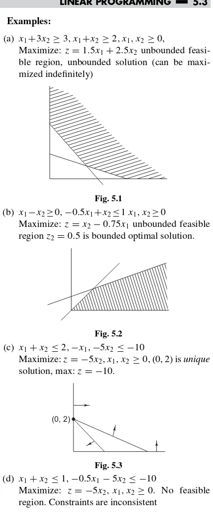
Examples:
(a) x1+3x2≥3, x1+x2 ≥2, x1, x2 ≥0,
Maximize:z=1.5x1+2.5x2 unbounded
feasi-ble region, unbounded solution (can be maxi-mized indefinitely)
Fig. 5.1
(b) x1−x2≥0,−0.5x1+x2≤1x1, x2≥0
Maximize:z=x2−0.75x1 unbounded feasible
regionz2 =0.5 is bounded optimal solution.
Fig. 5.2 (c) x1+x2≤2,−x1,−5x2≤ −10
Maximize:z= −5x2, x1, x2≥0, (0, 2) isunique
solution, max:z= −10.
(0, 2)
Fig. 5.3
(d) x1+x2≤1,−0.5x1−5x2≤ −10
Maximize: z= −5x2, x1, x2≥0. No feasible
Fig. 5.4 (e) 1.5x1+1.5x2≥9, x1+x2 ≤2.
No feasible region.
(0, 6)
(6, 0) (0, 2)
(2, 0)
WORKEDOUT EXAMPLES
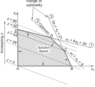
Example 1: ABC company produces two types of calculators. A business calculator requires 1 hour of wiring, one hour of testing and 3 hours of assem-bly, while a scientific calculator requires 4 hours of wiring, one hour of testing and one hour of assembly. A total of 24 hours of wiring, 21 hours of assembly and 9 hours of testing are available with the company. If the company makes a profit of Rs 4 on business calculator (BC) and Rs 10 on scientific calculator (SC), determine the best product mix to maximize the profit.
Solution: Let x1 be the number of business
cal-culators (BC) produced whilex2 be the number of
scientific calculators (SC) produced. Then the objec-tive is to maximize the profitz=4x1+10x2subject
to the following fine constraints:
x1+4x2≤24 (wiring) (I)
x1+x2≤9 (testing) (II)
3x1+x2 ≤21 (assembly) (III)
x1≥0 x2≥0
non negative (IV)
constraints (V)
To determine the feasible solution space consider the first quadrant of the x1x2-plane since x1≥0
andx2≥0. Then draw the straight linesx1+4x2=
24, x1+x2 =9 and 3x1+x2=2.1. Note that an
inequality divides thex1x2-plane into two open
half-space. Choose any reference point in the first quad-rant. If this reference point satisfies the inequality then the correct side of the inequality is the side on which the reference point lies. Generally origin (0, 0) is taken as the reference point. The correct side of the inequality is indicated by an arrow. The shaded region is the required feasible solution space satisfy-ing all the five constraints. The five corner points of the feasible region are A(0, 0), B(7, 0), C(6, 3), D(4, 5), E(0, 6). Identify the direction in whichzincreases without leaving the region. Arbitrarily choosingz= 0, 28, 54, 60, 66, observe that the straight lines (profit function)z=4x1+10x2orx2= −25x1+10z passes
through the corner points A, B, C, E, D respectively. The optimum solution occurs at the corner point D(4, 5), where the maximum value forz= 66 is attained. Thus the best product mix is to produce 4 business and 5 scientific calculator which gives a maximum profit of Rs. 66.
x2
Solution Space
3 +
= 21
x
x 1
2
x x 1
2 + 4
= 24
x
x
1 2
+ =
9 3
1 2
Range of optimality
Increasing
z
z
= 0
z
= 28
z
= 54E
z
= 60
z
= 66
A B
C D
x1
O ptim
um
Fig. 5.5
Example 2: (a) Solve the above problems to min-imizez= −4x1−10x2.
(b) Ifz=c1x1+c2x2, does an alternative optimal
solution exists
(c) Determine the range of optimality for the ratio
c1 c2
or c2
c1
Solution: (a) Rewriting,x2= −25x1−10z. Choose z=0,−28,−54,−60,−66, then the objective function passes through the corner points A, B, C, E, D respectively. Thus the minimum valuez= −66 is attained at the corner point D(4, 5). Observe that maximum ofz=4x1+10x2is 66 and minimum of z= −4x1−10x2is−66
i.e., maxf(x)= −min (−f(x)).
(b) Ifz=c1x1+c2x2coincides with the straight line
CD:x1+x2=9, then any point on the line segment
CD is an optimal solution to the current problem and thus has multiple (infinite) alternative optima. (c) Let z=c1x1+c2x2 be the objective function.
Then forc2=0, we write this as
x2= −c1
c2 x1+
z c2
The straight line
x1+4x2=24 rewritten as x2= −14x1+244 has
slope−14and the straight linex1+x2 =9 rewritten
asx2= −x1+9 has slope−1. Thus range of
opti-mality which will keep the present optimum solution valid is
1 4 ≤
c1 c2
≤1
Forc2 =4,1≤c1≤4
Similarly for c1=0, the range of optimality is
1≤ c2
c1 ≤4. Forc1=2,2≤c2≤8.
Example 3: The minimum fertilizer needed/hector is 120 kgs nitrogen, 100 kgs phosphorous and 80 kgs of potassium. Two brands of fertilizers available have the following composition.
Fertilizer Nitrogen Phos. Potassium Price/100 kgs bag A 20% 10% 10% Rs 50 B 10% 20% 10% Rs 40
Determine the number of bags of fertilizer A and B which will meet the minimum requirements such that the total cost is minimum.
Solution: LetXbe the number of bags of fertilizer A purchased andYbe the number of bags of fertilizer B purchased. Then the objective is to minimize the total cost =z=50X+40Y
subject to
20X+10Y ≥120 (Nitrogen)
10X+20Y ≥100 (Phosphorous)
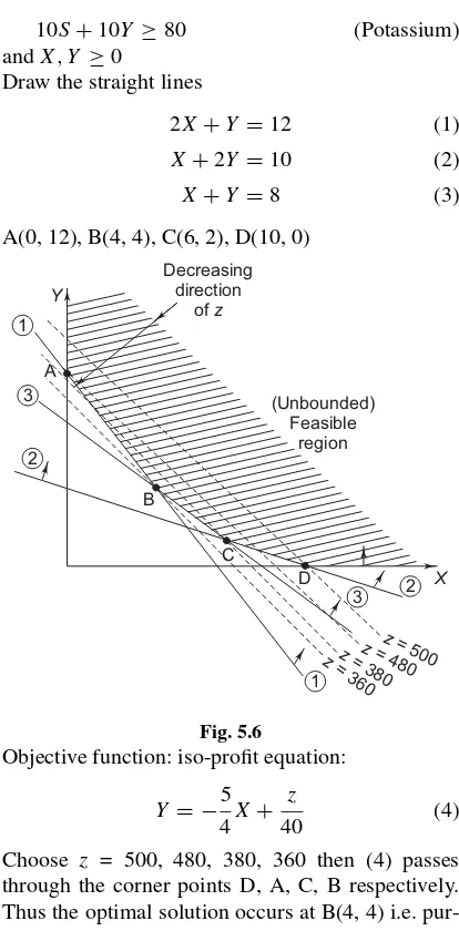
10S+10Y ≥80 (Potassium)
andX, Y ≥0
Draw the straight lines
2X+Y =12 (1)
X+2Y =10 (2)
X+Y =8 (3)
A(0, 12), B(4, 4), C(6, 2), D(10, 0)
X
2 2
3 3
1 1
z
= 500
z
= 480
z
= 380 z
= 360 C
B A
Y
Decreasing direction
ofz
(Unbounded) Feasible
region
D
Fig. 5.6
Objective function: iso-profit equation:
Y = −5
4X+ z
40 (4)
Choose z = 500, 480, 380, 360 then (4) passes through the corner points D, A, C, B respectively. Thus the optimal solution occurs at B(4, 4) i.e. pur-chase four bags of fertilizer A and 4 bags of fertilizer B with a total minimum cost of Rs 360/-.
EXERCISE
Solve the following LPP graphically:
for a profit of Rs 75/- determine the best product mix that will maximize the profit.
Chair Desk Available time Fabrication
Assembly Upholstery Linoleum
15 12 18.75
–
40 50 – 56.25
27,000 27,000 27,000 27,000
Ans: Produce 1000 chairs and 300 desks, making a profit of Rs 47,500.
Hint: Corner points are A(0, 0), B(1440, 0), C(1440, 135), D(1000, 300), E(250, 480), F(0, 480): Maximize:z= 25X+ 75Y. s.t.
15X+40Y ≤27,000,
12X+50Y ≤27000,
18.75X≤27000,56.25Y ≤27000
2. Asia paints produces two types of paints with the following requirements.
Standard Paint
Delux Paint
Total Available Quantity (in tons) Base
Chemicals Profit (in 100’s)
6 1 5
4 2 4
24 6
Determine the optimum (best) product mix of the paints that maximizes the total profit for the com-pany. Demand for deluxe paint can not exceed that of standard paint by more than 1 ton. Also maximum demand of deluxe paint is 2 tons.
Ans: Produce 3 tons of standard and 1.5 tons of deluxe paint, making a profit of Rs 2100.
Hint:Corner points: A(0, 0), B(4, 0), C(3, 1.5), D(2, 2), E(1, 2), F(0, 1); OF: Maximizez=5x1+
4x2subject to
6x1+4x2≤24, x1+2x2≤6,
−x1+x2≤1, x2≤2, x1, x2≥0.
3. In an oil refinery, two possible blending processes for which the inputs and outputs per production run are given below.
Process I II
Input Crude Crude
5 3
4 5
A B
Output Gasoline Gasoline
5 8
4 4
X Y
A maximum of 200 units of crude A and 150 units of crude B are available. It is required to produce at least 100 units of gasolineXand 80 units of gasolineY. The profit from process I is Rs 300 while from process II is Rs 400. Determine the optimal mix of the two processes.
Ans: Produce 30.7 units by process I and 11.5 units from process II, getting a maximum profit of Rs 13,846.20.
Hint:Maximize:z=300x1+400x2,subject to
5x1+4x2≤200,3x1+5x2≤150
5x1+4x2≥100,8x1+4x2≥80
Corner points: A(20, 0), B(40, 0), D(0, 30), E(0, 25), C400
13, 150
13
4. Minimize z=0.3x1+0.9x2 subject to x1+x2 ≥800, 0.21x1−0.30 x2≥0, 0.03x1− −0.01x2≥0,x1,x2≥0
Ans: x1=470.6, x2=329.4, minimum cost: Rs
437.64.
5. Maximize:z=30x1+20x2 subject tox1≤60, x2≤75, 10x1+8x2 ≤800.
Ans: x1=60,x2=25, Max: profit = Rs 2300
Hint:Corner points: A(0, 0), B(60, 0), C(60, 25), D(20, 75), E(0, 75).
6. Givenx1≥0,x2≥0,x1+2x2≤8, 2x1−x2≥ −2 solve to (a) maxx1(b) maxx2(c) minx1(d)
minx2(e) max 3x1+2x2(f) min−3x1−2x2(g)
max 2x1−2x2
Ans: (a)x1=8 (b)x2= 185 (c)x1 =0 (d)x2=0 (e)z
= 24,x1 =8,x2=0 (f)z= −24,x1=8,x2=0
(g)z= −285, x1= 45, x1 =185
7. Minimize z=x1+x2 s.t. x1≥0, x2≥0 2x1=x2 ≥12, 5x1+8x2≥74, x1+6x2≥28.
Ans: x1=2,x3=8, min. 10
8. Maximize:z=5x1+3x2s.t.x1≥0,x2≥0,
3x1+5x2 ≤15, 5x1+2x2≤10
Ans: x1 =1.053,x2 =2.368, Max: 12.37
Hint:Corner points: (0, 3), (1.053, 2.368), (2, 0) 9. Maximize: z=2x1−4x2 s.t. x1≥0, x2≥0,
3x1+5x2≥15, 4x1+9x2 ≤36
Ans: x1 =9,x2=0, Max: 18
Hint:Corner point: (0, 3), (0, 4), (5, 0) (9, 0) 10. Maximize: z=3x1+4x2 s.t. x1≥0, x2≥0,
2x1+x2≤40, 2x1+5x2≤180
Ans: x1 =2.5,x2 =35,z=147.5
Hint:Corner points: 0(0, 0), A(20, 0), B(2.5, 35), C(0, 36)
11. Minimizez=6000x1+4000x2s.t.x1≥0,x2 ≥
0, 3x1+x2≥40, x1+2.5x2≥22, x1+x2 ≥ 40
3.
Ans: x1 =12,x2 =4,zmin= 88,000
Hint:A(22, 0), B(12, 4), C(0, 40)
Note: Constraintx1+x2 ≥403 is redundant.
12. Maximize z=45x1+80x2 s.t. 5x1+20x2 ≤
400, 10x1+15x2≤450.
Ans: x1 =24,x2=14,z=Rs2200.
5.4 CANONICAL AND STANDARD FORMS OF LPP
Since max f(x)= −min (−f(x)), an LPP with maximation can be transferred to a minimization problem and vice versa. Thus, the following analysis can be applied for a maximization or minimization problem without any loss of generality.
Canonical formof LPP is an LPP given by (1) (2) (3) withallthe constraints (2) are of the less than or equal to type.
Standard formof LPP consists of (1) (2) (3) withall
constraints (2) are of theequalitytype and with all bi≥0, fori=1 tom.
Conversion to Standard Form Given any general LPP, it can be transformed to standard LPP as fol-lows:
1. In any constraint if the right hand side con-stantbi is negative, then multiply that constraint
throughout by−1. (Note that multiplication of an inequality constraint by−1, reverses, the inequal-ity sign i.e.−3<−2, multiplied by −1 we get (−1)(−3)>(−1)(−2) or 3>2.
2. A less than or equal to type constraint
j
aijxj ≤bi; (bi ≥0) gets transformed to an
equality
j
aijxj +si=bi
by the addition of a ’slack’ variablesi, which
is non negative.
3. A greater than or equal to type constraint
j
aijxj ≥bi; (bi ≥0)
can be transformed to an equality
aijxj−si =bi
by subtracting a ’surplus’ variableSi, which
is non negative. In general, it is more convenient to work with equations rather than with inequal-ities. So given any general LPP, convert it to a standard LPP, consisting of ’m’ simultaneous lin-ear equations in "n" unknown decision variables.
Minimize:
z=c1x1+c2x2+ · · · +cnxn(1)
subject to
a11x1+a12x2+ · · · +a1nxn=b1 a21x1+a22x2+ · · · +a2nxn=b2 − − − − − − − − − − − − − − −
am1x1+am2x2+ · · · +amnxn=bm
⎫ ⎪ ⎪ ⎬ ⎪ ⎪ ⎭
(2)
andx1, x2, x3,· · ·xn≥0 (3)
Herecj (Prices),bj (requirements) andai,j
(activity coefficients) fori=1 tom,j =lton) are known constants.
Ifm > n, discard them−nredundant equa-tions. Ifm=n, the problem may have a unique (single) solution which is of no interest since it can neither be maximized or minimized. If m < n, which ensures that none of the equations is redundant, then there may exist infinite number of solutions from which an optimal solution can be obtained.
Assume that m < n. Set arbitrarily any n−m variables equal to zero and solve the m equations for the remaining munknowns. Sup-pose the unique solution obtained be
{x1, x2,· · ·xm}, by setting the remaining
(n−m) variables
Basic solution
{x1, x2,· · ·, xm}is the solution of the system of
equa-tions (2) in whichn−mvariables are set to zero.
Basic variables
are the variablesx1, x2,· · ·, xmin the basic solution.
Basis
is the set ofmbasic variables in the basic solution.
Non-basic variables
xm+1, xm+2,· · ·xn are the (n−m) variables which
are equated to zero to solve them equations (2), (resulting in the basic solution).
Basic feasible solution
is a basic solution which satisfies the nonnegativity restrictions, (3) i.e. all basic variables are non nega-tive. (i.e.xj ≥0 forj =1,2,3,· · ·m)
Nondegenerate basic feasible solution
is a basic feasible solution in which all the basic vari-ables are positive (i.e.,xj >0 forj =1,2,3,· · ·m)
Optimal basic feasible solution
is a basic feasible solution which optimizes (in this case minimizes) the objective function (1).
Why Simplex Method
In an LPP withmequality constraints and n vari-ables withm < n, the number of basic solutions is ncm. For smallnandm, all the basic solutions
(cor-ner points) can be enumerated (listed out) and the optimal basic feasible solution can be determined.
Example:
Maximize:z=2x1+3x2s.t. 2x1+x2 ≤4,x1+
2x2≤5. Rewriting 2x1+x2+x3=4,x1+2x2+ x4=5. Herem=2,n=4,ncm=4c2=6 The six
basic solutions are: 1. (0, 0, 4, 5), Feasible (F), Non-degenerate (ND) andz= value of O.F = 0
2. (0, 4, 0, -3), NF (non feasible) 3. (0, 2.5, 1.5, 0),z= 7.5 F, ND
4. (2, 0, 0, 3),z= 4, F, ND 5. (5, 0, - 6, 0), NF 6. (1, 2, 0, 0),z=8,
Feasible nondegenerate and optimal.
However, even forn=20,m=10, the number of basic solutions to be investigated is 1,84,756, a large part of which are infeasible. It is proved that the set of feasible solutions to a LPP form a convex set (the line joining any two points of the set lies in the set) and the corner (extreme) points of the convex set are basic feasible solutions. If there is an optimal solution, it exists at one of these corner points. The simplex method devised by GB Dantzig is a power-ful procedure which investigates in a systematic way for optimal solution at these corner points which are finite in number.
Form=10,n=20, simplex method obtains the optimal in 15 steps, thus having an advantage of 92,378 to 1.
5.5 SIMPLEX METHOD
The simplex method is an algebraic iterative pro-cedure which solves any LPP exactly (not approxi-mately) or gives an indication of an unbounded solu-tion. Starting at an initial extreme point, it moves in a finite number of steps, betweenmand 2m, from one extreme point to the optimal extreme point. Con-sider the following LPP with ’m’ less than or equal to inequalities in ’n’ variables.
Maximizez=c1x1+c2x2+ · · · +cnxn
subject toa11x1+a12x2+ · · · +a1nxn≤b1 a21x1+a22x2+ · · · +a2nxm≤b2
. . . . am1xm1+am2x2+ · · · +amnxn≤bm
Introducing ’m’ slack variabless1,s2,. . .,sm, the
less than or equal to in equalities are converted to equations.
a11x1+a12x2+ · · · +a1nxn+s1=b1
a21x1+a22x2+ · · · +a2nxn+s2=b2
. . . .
am1x1+am2x2+ · · · +amnxn+ · · · +sm=bm
Herex1, x2,· · ·, xn, s1, s2,· · ·, smare all
Maximize:z=c1x1+ · · · +cnxn+0.s1+ · · · +
0.sm.
Thus there are m equations in m+n variables. Putting (m+n)−m=n variables zero we get a starting basic feasible solution. Take x1=x2= · · ·xn=0. Then the initial solution contains them
basic variabless1, s2· · ·, sm. This corresponds to the
corner point origin with value of the objective func-tion zero. Since this is a problem of maximizafunc-tion, the value of objective function will increase if we introduce one of non-basic variablexj (j =1 ton),
into the solution forcing out one of the basic variable. The obvious choice is thexj with the largestcj. Ties
are broken arbitrarily. The objective equation is writ-ten asz−c1x1−c2x2− · · · −cnxn+0.s1+ · · · +
0.sn=0
For efficient use, this data is written in the form of a table known as simplex tableau shown below:
Remark Basis Solution
-row 1 – – – – 0 0 0 0
-row 0 1 0 0
s -row 0 0 1
-row
-row 0 0 0 1
z x x x xn s s s
c z c c c c
s s a a a a b
s a a a a b
s a
s s a a a a b
1 2 1 2
1 2
1 1 11 12 1 1 1
2 2 21 22 2 2 2
1 2
j m
j n
j n
j n
i ij
m m m m mj mn m
1
¼
¼
¼
¼
¼
¼
¼
¼
¼
¼
¼
¼
¼
¼
¼
¼
¼
¼
¼
¼
¼
¼
¼
The first row, z-row contains the coefficients of the objective equation with last element in rectangle indicating the current value of the objective func-tion (In the present case it is zero). The left most (first) column indicates the current basic variables s1, s2,· · ·, sm. The right most (last) column is the
solution column. Thuss1=b1, s2 =b2,· · ·, sm= bm(all resources unused) is the basic solution with
the value of the objective function zero.
Test for optimality
Ifallthez-row coefficients of the nonbasic variables are nonnegative, then the current solution is optimal. Stop. Otherwise goto step I.
Step I.Entering variables: Suppose -cj, thez-row
coefficient of the non basic variablesxj is the most
negative, then the variablexjwill enter the basis. The jth column is known as the pivotal column. Step II.Leaving variable: Divide the solution col-umn with the corresponding elements of the pivotal column, with strictly positive denominator. Ignore the ratios, when the pivotal column elements are zero or negative.
Suppose bi
aij is the smallest non negative ratio among these ratios
bi
aij
, b2 a2j
,· · · bm
amj
,
then the basic variablesiwill leave the basis (and
therefore will become a non basic variable). Theith row is known as the pivotal row. The elementaij
at the intersection of the pivotal column and pivotal row is known as the pivotal element, which is encir-cled in the table step III. Compute the new simplex tableau with (s1, s2,· · ·, xj,· · ·, sm) as the new basis
compute. Pivot row:
New pivot row = current pivot rowpivot element .
All other rows including z:
New row = current row - (Corresponding pivot column coefficient)×(New pivot row).
The solution-column in the new tableau readily gives the new basic solution with new objective value (last element in thez-row). Now test for optimality. If yes, stop. Otherwise go to step I.
Optimality condition
Thenonbasicvariable having the most negative (pos-itive) coefficient coefficient in the z-row will be the entering variable in a maximization (minimization) problem. Ties are broken arbitrarily. When all thez -row coefficients of the non basic variables are non-negative (nonpositive) then the current solution is optimal.
Feasibility condition
Thus the simplex method can be summarized as follows:
Step 0.If all the constraints are less than or equal to type, introduce slack variables and determine the starting basic solution.
Step I.Using optimality condition, select the enter-ing variable. If no variable can enter the basis, stop. The current solution is optimal.
Step II.Using feasibility condition determine the leaving variable.
Step III.Compute the new basic solution (new sim-plex tableau) and go to step I.
Artificial Variable Technique
For a LPP in which all the constraints are less than or equal to type withbi ≥0, an all-slack, initial basic
feasible solution readily exists. However for prob-lems involving≥inequalities or equality constrains no such solution is possible. To alleviate this, artifi-cial variables are introduced in each of the≥or = type constraints, and slack variables for the less than or equal to type which will then provide a starting solution. The M-method and the two-phase method are two closely related methods involving artificial variables.
M-Method (also Known as Charne’s Method or Big M-Method)
Since artificial variables are undesirable, the coeffi-cient for the artificial variable in the objective func-tion is taken as−M in maximization problem and as + M in minimization problems. Here M is a very large positive (penalty) value. The augmented prob-lem is solved by simplex method, resulting in one of the following cases:
1. When all the artificial variables have left the basis and optimality condition is satisfied, then the cur-rent solution is optimal.
2. When one or more artificial variables are present in the basis at zero level and the optimality condi-tion is satisfied, then the solucondi-tion is optimal with some redundant constraints
3. No feasible solution exists when one or more arti-ficial variables are present in the basis at a positive level although the optimality condition is satis-fied. Such a solution is known aspseudo optimal solutionsince it satisfies the constraints but does not optimize the objective function.
Note: Since artificial variables which is forced out
of the basis, is never considered for reentry, the col-umn corresponding to the artificial variable may be omitted from the next simplex tableau.
Two-Phase Method
In the M-method, M must be assigned some specific numerical value which creates trouble of roundoff errors especially in computer calculations. The z-coefficient of the artificial variable will be of the form aM + b. For large chosen M, b may be lost and for small chosen M and small a, b may be present leading to incorrect results. The two phase method consists of two phases and alleviates the difficulty in the M-method.
Phase I
Exactly as in M-method, introduce necessary artifi-cial variables to get an initial basic feasible solution. Solve this augmented problem, by simplex method tominimize r, the sum of the artificial variables. If r=0, then all the artificial variables are forced out of the basis. Goto phase II. Ifr >0, indicating the presence of artificial variables at non zero level, LP has no feasible solution
Phase II
The feasible solution of phase I forms the initial basic feasible solution to the original problem (without any artificial variables). Apply simplex method to obtain the optimal solution.
WORKED OUT EXAMPLES
Enumeration
solutions. Find the optimal solution and the value of the objective function.
Maximizez= 2x1+3x2+4x3+7x4subject to
2x1+3x2−x3+4x4=8 x1−2x2+6x3−7x4= −3
andx1, x2, x3, x4≥0.
Solution: The number of equations m=2. The number of variablen=4. The number of basic vari-ables =m=2. The number of all possible solutions is4c2=6.
1. Put x3 =x4=0, solving 2x1+3x2=8, x1−
2x2= −3, we get x1=1, x2=2, z=8. Basic
feasible solution, not optimal, x1, x2 are basic
variables,x3,x2 are non basic variables (which
are always zero).
2. Put x2=x4=0. Solving 2x1−x3=8, x1+
6x3= −3, we getx1=1345, x3 = −143. Sincex3<
0, this is a basic non feasible solution.
3. Putx1=x4=0. Solving 3x2−x3=8,−2x2+
6x3= −3, we getx2=4516, x3= 167, z=16316. This
is a basic feasible solution (not optimal). 4. Put x3 =x2=0, solving 2x1+4x4=8, x1−
7x4= −3, we getx1= 229, x4=79, z=939, basic
feasible solution (not optimal).
5. Putx1=x3 =0. Solving 3x2+4x4=8, 2x2+
7x4=3 we getx2= 4413, x4=−137. This is a basic
non feasible solution.
6. Putx1=x2 =0. Solving−x3+4x4=8, 6x3−
7x4= −3, we getx3=4417, x4= 4517. Thus the
opti-mal basic feasible solution with the basic vari-ablesx3=4417, x4=4517 (and obviously the
remain-ing non basic variablesx1, x2at zero value) has
the maximum value of the objective function as
491 17.
Simplex Method: Maximization
Example 1: Solve the following LPP by simplex method.
Maximizez=2x1+3x2
subject to 2x1+4x2≤20
2x1+2x2≤12
4x1 ≤16 x1≥0, x2≥0
Solution: Introducing three slack variables, the given three less than or equal to inequality constraints will be expressed as equations. Assign zero cost to each of these slack variables. Then the standard form of the LPP is to
Maximizez=2x1+3x2+0·s1+0·s2+0·s3
subject to
2x1+4x2+s1 =20 2x1+2x2 +s2 =12 4x1 +s3=16
andx1, x2, s1, s2, s3≥0
Express the objective equation as
z−2x1−3x2 =0
Then the starting simplex tableau is represented as follows:
Basis Solution Remark
1 –2 –3 0 0 0 0 -row 0 2 4 1 0 0 20 -row 0 2 2 0 1 0 12 -row 0 4 0 0 0 1 16 -row
z x x s s s
z z
s s
s s
s s
1 2 1 2 3
1 1
2 2
3 3
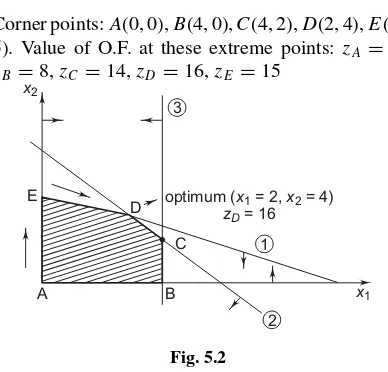
Corner points:A(0, 0),B(4, 0),C(4, 2),D(2, 4),E(0, 5). Value of O.F. at these extreme points: zA=0, zB =8,zC=14,zD =16,zE=15
2
x1
1 3
B A
E
x2
D optimum (zx= 161= 2,x2= 4)
D
C
Fig. 5.2
The initial basis consists of the three basic vari-abless1 =20,s2=12,s3=16. The two non basic
variables are listed in the left-most (first) column and their values (including the value of the objective function), in the right-most (last) column. Here the value of OF is 0 since all the resources are unutilized. In thez-row, the value of the objective function in the solution column is enclosed in a square. Since this is a maximization problem, to improve (increase) the value ofz, one of the non-basic variables will enter into the basis and there by forcing out one of the current basic variable from the basis (since the num-ber of basic variables in the basis is fixed and equals tom= 3 the number of constraints). From the opti-mality condition, the entering variable is one with the most negative coefficient in thez-row. In thez -row the most negative elements is−3. Thus the non basic variablex2will enter the basis. To determine the
leaving variable, calculate the ratios of the right-hand side of the equations (solution-column) to the corre-sponding constraint coefficients under the entering variablex2, as follows:
Basis Entering
Therefores1is the leaving variable. The value of
the entering variablex2in the new solution equals to
this minimum ratio 5. Heres1-row is the pivot row; x2 column is the pivot column and the intersection
of pivot column and pivot row is the pivot element 4 which is circled in the tableau. The new pivot row is obtained by dividing the current pivot row by the pivot element 4. Thus the new pivot row is
0
Recall that for all other rows, includingz-row, New row = current row−(corresponding pivot coefficient)×(new pivot row)
Newz-row = currentz-row−(−3) new pivot row
= currents3-row itself
= 0, 4, 0, 0, 0, 1, 16
Summarizing these results we get the new simplex tableau corresponding to the new basis (x2, s2, s3) as
follows. Note that this new basis corresponds to the corner point E(0, 5) with value of OF as 15.
Basis
From the tableau, the solution is
x2= 5,s2= 2,s3= 16 (basic variables)
x1= 0,s1= 0 (non basic variables), value of OF is
15.
Thus the solution moved from corner point A to corner point E in this one iteration. Optimal solution is not reached since all elements of z-row are not non negative. Since−12is the most negative element in the current z-row, the variablex1 will enter the
basis. To determine the leaving variable again calcu-late the ratios of RHS column with the elements of the entering variablex1.
1
Basis Entering Solution Ratio
x1
Therefore,s2will leave the basis. The pivotal
new simplex tableau corresponding to the new basis
Since all the elements in the current z-row are non-negative, the current solution is optimal. Read the solution from the tableau as
x2= 4,x1= 2,s3= 8 (basic variables)
s1= 0,s2= 0 (non basic variables)
value of O. F is 16.
Note that this solution corresponds to the corner point D(2, 4). In this second iteration solution moved from E to D.
Simplex Method: Minimization:
Example 1: Minimize:z=x1+x2+x3 subject
tox1−x4−2x6 =5, x2+2x4−3x5+x6=3, x3+2x4−5x5+6x6=5.
Solution: Fortunately the problem contains already a starting basic feasible solution withx1,x2,x3as the
Example 1: Solve LPP by simplex method. Maximize:z=2x1−3x2+4x3+x4subject to x1+5x2+9x3−6x4≥ −2
3x1−x2+x3+3x4 ≤10 −2x1−3x2+7x3−8x4≥0
andx1, x2, x3, x4≥0.
Solution: Rewriting in the standard form
Objective equation is:z−2x1+3x2−4x3−x4=0
The first simplex tableau with the 3 basic variables x5, x6, x7is given below:
Since−4 is most negative element in thez-row, the associated variablex3will enter the basis. Out of the
three ratios−29,101,−07, the first and third are ignored (because the denominator is negative). Sox6 will
be outgoing variable. The pivotal element is 1. So pivotal row remains same. The next simplex tableau withx5, x3, x7is given below.
In the currentz-row,x2has the most negative
coef-ficient−1, so normallyx2 should enter the basis.
However, all the constraint coefficients underx2are
negative, meaning thatx2 can be increased
indefi-nitely without violating any of the constraints. Thus the problem has no bounded solution.
M-method:
Example 1: Solve the LPP by M-method minimizez=3x1+2.5x2
subject to 2x1+4x2≥40
3x1+2x2≥50 x1, x2≥0
Solution: Introducing surplus variablesx3, x4, the
greater than inequations are converted to equations. Minimizez=3x1+2.5x2+0·x3+0·x4
subject to
2x1+4x2−x3=40
3x1+2x2−x4=50 x1, x2, x3, x4≥0
In order to have a starting solution, introduce two artificial variablesR1andR2in the first and second
equations. In the objective function the cost coeffi-cients for these undesirable artificial variablesR1and R2 are taken as a very large penalty value M. Thus
the LPP takes the following form:
Minimizez=3x1+2.5x2+0·x3+0·x4+
The z-column is omitted in the tableau for conve-nience because it does not change in all the iterations. Solving (2) and (3) we get
R1=40−2x1−4x2+x3 (4)
and R2=50−3x1−2x2+x4 (5)
Substituting (4) and (5) in the objective function (1) we get
which is independent ofR1andR2. Thus the
objec-tion equaobjec-tion is
z−(3−5M)x1−(2.5−6M)x2−Mx3− −Mx4=90M
The simplex tableau with the starting basic solution containingR1andR2as the basic variables in given
below:
In the z-row, the most positive coefficient is
−2.5+6M. Sox2 will be entering variable. Since 40
4 =10, 50
basis. So 4 is the pivotal element. New simplex tableau is given below:
Basis x1 x2 x3 x4 R1 R2 Solution row, the variablex1will enter the basis forcingR2out
since the minimum of the ratios101 2
=20,302 =15 is
15. So pivotal element is 2. The next simplex tableau is shown below:
15
Since all the elements in thez-row are non posi-tive, the current solution is optimal given byx1=15, x2= 52with value of objective function2054 (observe
that the artificial variablesR1,R2and surplus
vari-ablesx3, x4 are nonbasic variables assuming zero
values. Thus R1, R2 have been forced out of the
basis).
Two-Phase Method
Example 1: Solve LPP by two-phase method Maximizez=2x1+3x2−5x3
subject to x1+x2+x3=7
2x1−5x2+x3≥10
andx1, x2, x3≥0
Solution: Phase I: Introducing a surplus variable x4and two artificial variablesR1 andR2, the Phase
I of the LPP takes the following form:
Minimize r=R1+R2 (1)
Substituting (4), (5) in (1) we get the objection func-tion as
Minimize r=(7−x1−x2−x3)+(10−2x1+
5x2−x3+x4)
or Minimize r= −3x1+4x2−2x3+x4+17 or r+3x1−4x2+2x3−x4 =17
The simplex tableau containing the basic solution withR1,R2as the basic variables is given below.
Basis x1 x2 x3 R1 R2 x4 Solution
The variablex1will enter the basis since 3 is most
positive coefficient in ther-row of this minimization problem. The variableR2will leave the basis since
10
2 =5 is less than 7
1 =7. The pivotal element is 2.
Dividing the pivot row by the pivot element 2, we get the new pivot row as 1,−52, 12, 0, 12,−12, 5. Here the newrth-row:
=(3−4 2 0 0−1 17)−31−52 120 12−12 5
The new simplex table withR1andx1 as the basic
variables is shown below:
Basis x1 x2 x3 R1 R2 x4 Solution
the basis pushing outR1 with ratio 2
other ratio 5
−52 is ignored since the denominator is negative). The pivotal element is72. The pivot row is
The next simplex tableau of the second iteration with x1andx2as the basic variables is given below.
Basis x1 x2 x3 R1 R2 x4 Solution
The phase I is complete sinceris minimized attain-ing value 0, producattain-ing the basicfeasible solutionx1
=457,x2=47. Note that both the artificial variablesR1
andR2have been forced out of the (starting) basis.
Therefore the columns ofR1 andR2can altogether
be ignored in the future simplex tableau.
Phase II: Having deleted the artificial variables R1andR2and having obtained a basic feasible
solu-tionx1, x2 we solve theoriginal problemgiven by
maximization ofz=2x1+3x2−5x3
subject to
x2+17x3+17x4= 47 x1+67x3−17x4= 457
andx1, x2, x3, x4≥0
The tableau associated with this phase II is
Basis x1 x2 x3 x4 Solution
Sincex2with most negative element in thez-row is
already in the basis, the current solution is optimal. The basic feasible solution isx1=457, x2 =47 and
the maximum value of the objective function is1027 .
5.6 LINEAR PROGRAMMING PROBLEM
EXERCISE
Enumeration:
1. If a person requires 3000 calories and 100 gms of protein per day find the optimal product mix of food items whose contents and costs are given below such that the total cost is minimum. Formu-late this as an LPP. Enumerate all possible solu-tions. Identify basic, feasible, nonfeasible, degen-erate, non degenerate solutions and optimal solu-tion.
basic solutions: F = Feasible, NF: non-feasible, D: degenerate, ND: non degenerate
1. x1= 109, x2= 272, z= 1107 , F, ND
2. Find all basic solutions for
x1+2x2+x3=4,2x1+x2+5x3 =5
Ans: (2, 1, 0) F, ND; (5, 0,−1), NF, ND;
0,53,23F, ND.
3. Find the optimal solution by enumeration Max:z=5x1+10x2+12x3
s.t.x1, x2, x3 ≥0,
15x1+10x2+10x3≤200,10x1+25x2+
20x3 =300
Ans: 1. (7.27,9.1,0,0),z=127·27 2. (5,0,12.5,0),z= 175 3. (30,0,0,−250), NF 4. (0,−20,40,0), NF 5. (0, 12, 0, 80),z= 120 6. (0, 0, 15, 50),z= 180 (1) (2) (5) are F, ND: (6) is optimal solution;
4. Find the optimal solution by enumeration Max: z=2x1+3x2 s.t. 2x1+x2≤4, x1, x2 ≥
0, x1+2x2 ≤5.
Ans: 1. (0, 0, 4, 5),z=0, F, ND 2. (0,4,0,−3) NF
3. (0,2.5,1.5,0), z=7.5, F, ND 4. (2, 0, 0, 3),z=4, F, ND 5. (5,0,−6,0), NF
6. (1, 2, 0, 0),z=8, F, ND, optimal.
Simplex Method
Solve the following LPP by simplex method.
1. A firm can produce 5 different products using 3 different input quantities, as follows.
Input Technical coefficients Capacity
quantity 1 2 3 4 5
A 1 2 1 0 1 100
B 0 1 1 1 1 80
C 1 0 1 1 0 50
Profit 2 1 3 1 2
Maximize the profit
Ans: x1 =20, x3=30, x5=50, profit: Rs = 30
Hint: Max:z=2x1+x2+3x3+x4+2x5 s.t. x1+2x2+x3+x5≤100;x2+x3+x4+x5≤
80;x1+x3+x4≤50
2. Max: z=2x1+x2 s.t. x1, x2≥0; 3x1+5x2≤
15; 6x1+2x2≤24.
Ans: x1=154, x2=34, z=334
3. Max:z=3x1+4x2+x3+7x4s.t. 8x1+3x2+
4x3+x4≤7,
2x1+6x2+x3+5x4≤3, x1+4x2+5x3+2x4≤8 x1, x2, x3, x4≥0.
Ans: x1=1619, x4=195, x7=12619, z= 8319
4. Minimizez=x2−3x2+2x5
s.t.x1+3x2−x3+2x5 =7, −2x2+4x3+x4=12, −4x2+3x3+8x5+x6 =10
Ans: x2=4, x3=5, x6 =11, z= −11
5. Max:z=2x1+5x2+4x3
s.t.x1+2x2+x3≤4;x1+2x2+2x3≤6
Ans: x2=1, x3=2, z=13
6. Max:z=5x1+4x2s.t.,x1, x2≥0;
6x1+4x2≤24;x1+2x2≤6, x1−x2≥ −1;−x2≥ −2
Ans: x1=3,x2= 32,z= 21
7. Max: z=x1+2x2+x3 s.t. x1, x2, x3≥0,
2x1+x2−x3≤2;−2x1+x2−5x3≥ −6;
4x1+x2+x3≤6.
Ans: x2=4, x3=2, x6 =0, z= −10
(Note: Degenerate solution) 8. Max:z= −x1+3x2−2x3s.t.
3x1−x2+2x3≤7,2x1−4x2≥ −12;
4x1−3x2−8x3≥ −10;x1, x2, x3≥0.
Ans: x1=4, x2=5, z=11
9. Max.z=6x1+9x2s.t.x1, x2≥0,2x1+2x2≤
24;x1+5x2≤44,6x1+2x2≤60
Ans: x1=4, x2=8, x6 =20, z=96
Multiple optima:
10. Minimize:z= −x1−x2s.t.x1, x2≥0 x1+x2≤2, x1−x2≤1, x2≤1
Also another optimal solution is x1=1, x2=
1, z= −2
11. Max: z=6x1+4x2 s.t. x1, x2 ≥0, x1≤
4,2x2≤12,3x1+2x2≤18
Ans: x1 =4, x2=3, z=36
Another optimal solution: x1=2, x2 =6, z=
36
Unbounded solution
12. Max:z=4x1+x2+3x3+5x4s.t.
3x1−2x2+4x3+x4≤10,
8x1−3x2+3x3+2x4≤20, −4x1+6x2+5x3−4x4≤20
Ans: Unbounded solution
Note:In the second simplex tableau, sincex2has
most negative coefficient inz-row, normallyx2
should enter the basis. But all the entries in the column underx2are negative or zero. Sono
vari-able can leave the basis. Hence the solution isnot
bounded
13. Min:z= −3x1−2x2 s.t.x1, x2≥0, x1−x2 ≤
1,3x1−2x2≤6.
Ans: Unbounded solution
Note:In the 3rd simplex tableau,x3 having the
most positive value (12) inz-row should normally enter the basis. Butallthe entries underx3 are
negative. So OF can be decreased indefinitely.
M-Method
14. Minimize:z=4x1+2x2s.t. x1, x2≥0, 3x1+ x2 ≥27;−x1−x2≤ −21, x1+2x2≥30.
Ans: x1 =3, x2=18, z=48
15. Max:z=x1+2x2+3x3−x4s.t.
x1+2x2+3x3=15,2x1+x2+5x3 =20, x1+2x2+x3+x4=10, x1, x2, x3, x4≥0
Ans: x1 =x2=x3= 52,x4=0, z=15
16. Min: z=2x1+x2 s.t. x1, x2≥0, 3x1+x2=
3,4x1+3x2≥6, x1+2x2 ≤3
Ans: x1 =35, x2= 65, z= −125
17. Min: z=3x1−x2 s.t. x1, x2 ≥0,2x1+x2≥
2;x1+3x2≤3;x2≤4
Ans: x1=3, x3=4, x6 =4, z=9
18. Max: z=x1+5x2 s.t. x1, x2≥0,3x1+4x2≤
6;x1+3x2≥2
Ans: x2= 32, x4 =52, z= −152
19. Min: z=2x1+4x2+x3 s.t. x1+2x2−x3≤
5; 2x1−x2+2x3 =2;−x1+2x2+2x3≥1
Ans: x3=1, x4=6, x6 =1, z=1
Two-Phase Method:
20. Max:z=x1+5x2+3x3s.t.x1, x2, x3≥0, and x1+2x2+x3=3; 2x1−x2=4
Ans: (2, 0, 1),z= 5
21. Min: z=4x1+x2 s.t. x1, x2, x3, x4≥0, and
3x1+x2=3; 4x1+3x2 ≥6, x1+2x2≤4.
Ans: 2 5,
9 5,1,0
, z= 175
22. Minimize z=7.5x1−3x2 s.t. x1, x2, x3≥
0,3x1−x2−x3≥3;x1−x2+x3 ≥2
Ans: x1=54,x2= 0,x3= 34, z= 758
23. Minimize z=3x1+2x2, s.t. x1, x2,≥0, x1+ x2≥2;x1+3x2≤3, x1−x2=1
Ans: x1=32;x2=12, z=112
24. Minimize: z=5x1−6x2−7x3 s.t.x1+5x2−
3x3≥15; 5x1−6x2+10x3≤20; x1+x2+ x3=5,x1, x2, x3≥0
Ans: x2= 154;x3= 54, x5=30, z= −1254
25. Max:z=2x1+x2+x3s.t.
4x1+6x2+3x3≤8;
3x1−6x2−4x3≤1; 2x1+3x2−5x3≥4; x1, x2, x3≥0
5.7 THE TRANSPORTATION PROBLEM
The transportation problem is a special class of Lin-ear programming problem. It is one of the Lin-earliest and most useful application of linear programming problem. It is credited to Hitchcock, Koopmans and Kantorovich. The transportation model consists of transporting (or shipping) a homogeneous product from ‘m’ sources (or origins) to ‘n’ destinations, with the objective of minimizing the total cost of trans-portation, while satisfying the supply and demand limits.
Let ai denote the amount of supply at the ith
source,bj denote the demand at destination j;cij
denote the cost of transportation per unit fromith source tojth destination;xij the amount shipped
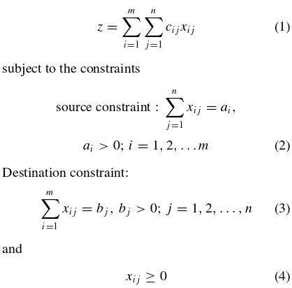
from originito destinationj. Then the transportation problem is to minimize the total cost of transporta-tion
z= m
i=1 n
j=1
cijxij (1)
subject to the constraints
source constraint :
n
j=1
xij =ai,
ai >0;i=1,2, . . . m (2)
Destination constraint:
m
i=1
xij =bj, bj >0;j =1,2, . . . , n (3)
and
xij ≥0 (4)
In the balanced transportation problem it is assumed that the total quantity required at the destinations is precisely the same as the amount available at the origins i.e.
m
i=1 ai=
n
j=1
bj. (5)
(5) is the necessary and sufficient condition for the existance of a feasible solution to (2) and (3).
Denoting the sources and destinations as nodes and routes as arcs, the transportation problem can be represented as a network shown below:
Sm Dn
S1 D1 b1
a1
b2 a2
bn
am
S2 D2
Demand Destinations
Sources Supply
c11;x11
cmn;xmn
The system of equations (1) to (4) is a linear pro-gramming problem withm+nequations inmn vari-ables. The transportation problem always has a finite minimum feasible solution and an optimal solution containsm+n−1 positivexij’s when there arem
origins andndestinations. It is degenerate if less than m+n−1 of thexij’s are positive. No transportation
problem has ever been known to cycle. Table for Transportation Problem
S1
S2
Si
Sm
bj
a
a 1
2
ai
am
bn
bj
b2
b1 Sai=
Sbj
c1n
c1j
c12 c11
cmn
cmj
cm2
cm1
x1n
x1j
x12 x11
xmn
xmj
xm2
xm1
K
K
ai
Dn
Dj
D2
D1 K K
Destinations
Sources
Note: Zero values for nonbasic variables are not
filled while zero values for basic variables are shown in the tableau.
Determination of Initial (starting) Basic Fea-sible Solution
An initial basic feasible solution containingm+n−
1 basic variables can be obtained by any one of the following methods (a) the north west corner rule (b) row minimum (c) column minimum (d) matrix minimum (or least cost method) (e) Vogel approx-imation method. In general, Vogel’s method gives the best starting solution. Although computationally north west corner rule is simple, the basic feasible solution obtained by this method may be far from optimal since the costs are completely ignored.
(a) North-west corner rule (due to Dantzig):
Step I:Allocate as much as possible to the north west corner cell (1, 1). Thus letx11=min(a1, b1). Ifa1≤ b1 thenx11 =a1and allx1j =0 forj =2,3, . . . n
i.e. exceptx11all other elements of the first row are
zero. The first row is satisfied so cross out the first row and move tox21of second row.
Ifa1≥b1 thenx11 =b1 and allxi1=0 fori=
2,3, . . . mi.e., exceptx11 all other elements in the
first column are zero. The first column is satisfied so cross out the first column and move tox12of the
second column.
Note: If both a row and column are satisfied (i.e.,
say x11=a1=b1) simultaneously, then cross out
either row or column only butnot bothrow and col-umn.
Step II:Allocating as much as possible to the cell (2, 1) or (1, 2) cross out the row or column and move to (3, 1) or (1, 3).
Step III: If exactly one row or column is left uncrossed out, stop. Otherwise go to step II wherein move to lower row (below) if a row has just been crossed out or move to right column if a column has just been crossed out.
Note: Cells from “crossed out” row or column can
not be chosen for basis cells at a later step in the determination of starting basic solution.
(b) Row-minimum
Identify the minimum cost elementc1k in the first
row. (Ties are broken arbitrarily). Allocate as much as possible to cell (1,k). Ifa1≤bkthenx1k=a1so
move to the second row after changingbktobk−a1.
Identify the minimum element in second row and allocate as much as possible. Continue this process until all rows are exhausted. Ifa1> bkthenx11=bk,
changea1toa1−bk, and identify the next smallest
(minimum) element in the first row allocate, continue the process until the first row is completely satisfied.
(c) Column-minimum
This is exact parallel to the above row-minimum method except that minimum in the columns are identified instead of rows.
(d) Matrix minimum (least-cost method):
Identify the least (minimum) element cij in the
entire matrix. (Ties are broken arbitrarily). Allocate as much as possible to the (i, j)th cell. If ai ≤bj
thenxij =ai, changebj tobj−ai. Ifai ≥bj then xij =bj, changeaitoai−bj. Identify the next least
element and allocate as much as possible. Continue this process until all the elements in the matrix are allocated (satisfied).
(e) Vogel approximation method
Step I.The row penalty for a row is obtained by sub-tracting thesmallestcost element in that row from thenext smallestcost element in the same row. Cal-culate the row penalties for each row and similarly column penalties for each column.
Step III.
(a) A starting solution is obtained when exactly one row or one column with zero supply or demand remains uncrossed out. Stop.
(b) Determine the basic variables in an uncrossed row (column) with positive (non zero) supply (demand) by the least-cost method. Stop. (c) Determine the zero basic variables in all the
uncrossed out rows and columns having zero sup-ply and demand by the least cost method. Stop. (d) Otherwise, go to step 1, recalculate the row and
column penalties and go to step II.
Note: Vogel’s method, which is a generalization of
the matrix minimum (least cost method) gives better solution in most cases than all the other methods listed above.
Method of Multipliers
The optimal solution to the transportation prob-lem is obtained by iterative computions using the method of multipliers (also known asU V-method or stepping-stone method or MODI (modified distri-bution) method). First of all, obtain a starting initial basic feasible solution containingm+n−1 basic variables (by any one of the above methods).
Step I:Introduce unknownsuiwith rowiandvjwith
columnjsuch that for each current basic variablexij
in the tableau,
ui+vj =cij
is satisfied. This results inm+nequations inm+n unknowns. Assume thatu1=1 (oru1=0). (Instead
ofu1, any other variableui orvj can be chosen as
zero or one, resulting in the same optimal solution but with different values in the tableau). Solving the equations inui,vj we getui fori=1 tomandvj
forj =1 ton.
Step II.For each non basic variable, compute cij =ui+vj −cij
Step III:(a) Ifcij ≤0 for anyi andj (i.e. for all
non basic variables), stop. The current tableau gives the optimal solution withminimumcost.
(b) Ifcij >0, then solution is to be revised. The entering variableis one which has most positivecij
(i.e., maxcij for alliandj).
(c) The leaving variableis determined by con-structing a closedθ-loop which starts and ends at the entering variable and consists of connected horizon-tal and vertical lines (without any diagonals). Thus each corner of the loop lies in the basic cell, except the starting cell. The unknownθ is subtracted and added alternatively at the successive corners so as to adjust the supply and demand. From the cells in whichθ is subtracted, choose the maximum value ofθsuch thatxij −θ≥0. This feasibility condition
determines the leaving variable. Now go to step I.
MaximizationA transportation problem in which the objective is to maximize (the profit) can be trans-fered to a minimization problem by subtracting all the entries of the cost matrix from the largest entry of the matrix.
Unbalanced problemin which the total supply is not equal to the total demand can always be trans-fered to a balanced transportation problem by aug-menting it with a dummy source or dummy destina-tion. A dummy destination is added when supply is greater than the demand. The cost of transportation from any source to this dummy destination is taken as zero. Similarly when demand is greater than sup-ply, a dummy source is added. The cost of shipping from this dummy source to any destination is taken as zero. Now the corresponding balanced problem is solved by the method of multipliers.
Transhipment problemconsists of transporting from source to destination via (through) intermedi-ate or transient nodes, known astranshipment nodes
prob-lem can be transformed to a regular transportation problem as follows:
I. Identify the pure supply nodes, pure demand nodes and transhipment nodes from the given net-work.
II. Denote the pure supply nodes and transhipment nodes as the sources.
III. Denote the pure demand nodes and transhipment nodes as the destinations.
IV. Note down the transportation costscij read from
the given network. Ifith source is not connected to jth destination, putcij =MwhereMis a large
(penalty) value. Takecii =0 since it costs zero
for transporting fromith source to itself (ith des-tination).
V. Identify supply at a pure supply node as the origi-nal supply; demand at a pure demand node as the original demand; supply at a transhipment node as the sum of original supply and buffer and finally demand at a transhipment node as the sum of the original demand and buffer.
Now the above transformed regular transportation problem can be solved by using the method of mul-tipliers.
Degeneracy The solution of a transport problem is said to be degenerate when the number of basic variables in the solution is less thanm+n−1. In such cases, assign a small valueεto as many non-basic variables as needed to augment tom+n−1 variables. The problem is solved in the usual way treating the ε cells as basic cells. As soon as the optimum solution is obtained, letε→0.
5.8 Transportation Problem
WORKEDOUT EXAMPLES
Starting Solution:
Example 1: Obtain a (non artificial) starting basic solution to the following transportation problem using (a) North west corner rule (b) Row-minimum (c) Column minimum (d) Least cost (Matrix minima)
(e) Vogel’s (approximation) method
S
S
S
1
2
3
0 2
1 4 3
2 2 4
0
D1 D2 D3
7 6 6
8
5
6
Solution:
(a) NWCR:
S
S
S
1
2
3
0
2
1 4
3
2 2
4
0
D1 D2 D3
7 6, 5 6 8, 1
5
6
7 1
5
6
Supply as much as possible to the north-west corner cell (1, 1).
Cost: 7×0+1×4+5×3+6×0=19
Note: This is a degenerate solution because it
con-tains only 4 basic variables (instead of 3+3−1=5 basic variables).
(b) Row Minimum
S
S
S
1
2
3
0
2
1 4
3
2 2
4
0
D1 D2 D3
7 6, 1 6, 5 8, 1
5
6
7 1
1 5
5 1
Allot as much as possible in the first row to the cell with least (minimum) cost i.e. (1, 1). The balance allot to the next least cell in the first row.
Cost: 7×0+1×2+5×3+1×2+5×0=
19
Note: This is a non-degenerate solution (since it
(c) Column Minimum This is a degenerate solution containing 4 basic variables.
(d) Least cost method (matrix minima)
S
Allot as much possible to that cell which has least cost in the entire matrix say (1, 1) (tie broken arbi-trarily between (1, 1) and (3, 3).
Cost: 7×0+1×4+5×3+6×0=19 This is a degenerate solution.
(e) Vogel’s (approximation) method
S
penalties 1 1 1
This is a non-degenerate solution.
Method of Multipliers
Example 1: Solve the following transportation problem byU V-method obtaining the initial basic solution by (a) Vogel’s method (b) NWCR (c) com-pare the number of iterations in (a) and (b).
S
(a) Initial solution by Vogel’s method
P
Thus the initial basic feasible solution by Vogel’s method is given by
S
where the basic variables are circled
Total cost: (20×0)+(10×2)+(10×0)+
(10×1)+(25×0)+(25×0)=30
jsuch that for each basic variablexij we have ui+vj =xij
Arbitrarily choosing u1 =1 we solve for the
remainingui,vj’s as follows:
Basic variable u,vequation solution x13 u1+v3=0 v3= −1
Now usingui andvj the non basic variables are
calculated as
Non basic variables are placed in the south east corner of each cell. Then the new table is
S
During computation, it is not necessary to writeu, vequations and solve them explicitly. Instead, choos-ingu1=1, computev3,v4from the basic variables x13,x14in the first row. Now usingv4,u3is obtained
from the basic variablex34. Similarlyu2is obtained
usingv3from the basic variablex23. Now usingu2
we getv1and finally usingu3we getv2.
Incoming: Amongst the nonbasic variables, the
enteringvariable is the one with themost positive
value (in the south east corner of the cell). Thusx21
will be the entering variable.
Outgoing: The leaving (basic) variable is deter-mined by constructing a closedθ-loop which starts and ends at the entering variablex21. In this modified
distribution all variables should be nonnegative and supply and demand satisfied. Then
x14 =10−θ≥0
x22 =25−θ≥0
The maximum value ofθ is 10 (which keeps both x14, x22 nonnegative i.e., x14 =0, x22=15>0).
Thus the new table is
S
are all negative, the current table is the optimal. The optimal solution with least cost is (10×1)+(20×
0)+(10×0)+(10×1)+(15×0)+(35×0)=20.
ByU V method withu1=1 we get
Then the new table is
3
incoming andx33will be outgoing variable resulting
in the following table.
3
incoming with new following table which is the opti-mal solution since allxij =ui+vj −cij ≤0.
optimal cost is 20. Optimal solution isx12=10, x13=20,x21 =10,x23 =10,x32 =15,x34=35.
(c) The number of iterations is less when the initial solution is obtained by Vogel’s method.
Unbalanced Transportation Problem
Example 1: Three electric power plantsP1,P2,P3
with capacities of 25, 40 and 30 kWh supply electric-ity to three citesC1,C2,C3. The maximum demand
at the three cities are estimated at 30, 35 and 25 kWh. The price per kWh at the three cites is given in the following table
During the month of August, there is a 20% increase in demand at each of the three cities, which can be met by purchasing electricity from another plantP4 at a premium rate of Rs 1000/- per kWh.
plant 4 is not linked to city 3. Determine the most economical plane for the distribution and purchase of additional energy. Determine the cost of additional power purchased by each of the three cities.
Solution:
Apply Vogel’s method to obtain the initial solution. For all nonbasic variables ui+vj−cij ≤0. The
present table is optimal. The optimal solution is P1C3: 25, P2C1=23, P2C2=17, P3C2 =25, P3C3=5,P4C1=13.
Total cost: Rs 36,710 + Rs 13000 = Rs 49710 only cityC1purchases an additional 13 kWh power from
P
Example 1: The unit shipping costs through the routes from nodes 1 and 2 to nodes 5 and 6 via nodes 3 and 4 are given in the following network. Solve the transhipment model to find how the shipments are made from the sources to destinations.
1
Solution: The entire supply of 300 units is tran-shipped from nodesP1 andP2 through T3 andT4
ultimately to destination nodesD5andD6. HereP1, P2 are pure supply nodes; T3, T4, D5 are
tranship-ment nodes;D6is pure demand node. The
tranship-ment model gets converted to a regular transportation problem with 5 sourcesP1, P2, T3, T4, D5and 4
des-tinationsT3, T4, D5andD6. The buffer amount B =
total supply ( or demand) = 100 + 200 = (or 150 +
150) = 300 units. A high penalty costMis associated with cellcijwhen there isnoroute fromith origin to
thejth destination. Zero cost is associated with cells (i, i) which do not transfer to itself. The initial solu-tion is obtained by Vogel’s method. Takingu1= 0 and M= 99 and applying method of multipliers we have
P
300 300 450 150
q
value of objective function is Rs 2650. Not allcij ≤
0. Note thatc43=92 is most positive so the variable x43will enter into the basis. To determine the variable
leaving the basis, constructθ-loop from cells (4, 3) to (2, 3) to (2, 2) to (4, 2). Chooseθ= 0 to maintain feasibility. Adjustingθ = 0, the leaving variable is x23. Thus the new tableau is
300 300 150 150
value of objective function is Rs 2650. Not all cij ≤0. Note that c31 =2 is most positive. Sox31
variable construct aθ-loop from cells (3, 1) to (2, 1) to (2, 2), to (4, 2) to (4, 3) to (3, 3) to (3, 1). Choose maximum value of θ = 200. Then x21 will be the
leaving variable. Adjustingθ= 200, the new tableau is given below.
p
300 300 450 150
Observe that all cij ≤0. Therefore the current
tableau is optimal. The basic feasible optimal solution is x11=100, x22=200, x31 =200, x33=
100, x42=100, x43=200, x53 =150, x54=150.
The value of the objective function is (100×1)+(200×2)+(200×0)+(100×6)+
(100×0)+(200×5)+(150×0)+(150×1) = 2250
Maximization:
Example 1: Solve the following transportation problem to maximize the profit.
D1 D2 D3
Solution: To transform this problem to a minimiza-tion, subtract all the cost entries in the matrix from the largest cost entry 8. Then the relative loss matrix is
Applying vogel’s method we get max penalty 3. So allocate to (1, 3).
P
Allocate to (1, 1) since 4 is the largest penalty
P
Allocate to (3, 2) since 3 is the largest penalty.
P
The maximum profit (wrt the original cost matrix) is (1×5)+(11×8)+(8×2)+(6×4)+
Degeneracy
Example 1: Solve the following TP using NWCR
0
Solution: By NWC rule
0
This is a degenerate solution since it contains only 4 basic variables (instead of 3 + 3 - 1 = 5 basic vari-ables). To get rid of degeneracy, introduce any one non-basic variable say in cell (3, 2) at ’ε’ level where εis a small quantity. Thus
0
since allcij ≤0 current solution is optimal. Now
lettingε→0 we get the solution asx11 =7, x12=
1, x22=5, x32=0, x33 =6 with OF = 19+2·ε=
19 asε→0
5.9 TRANSPORTATION PROBLEM
EXERCISE
1. Obtain the starting solution (and the correspond-ing cost i.e. value of objective function: OF)